Force Sensitive Resistor Gait

Detection And Severity Prediction From Gait

Imanne El Maachia, Guillaume-Alexandre Bilodeaua, Wassim Bouachirb

Apolytechnique Montreal,

2900 boul. Edouard Montpetit, Montreal (Qc), H3T 1J4, Canada 5800 rue Saint-Denis, bur. 1105, Montreal (Qc), H2S 3L5, Canada

Abstract

Diagnosing Parkinson’s disease is a complex task that requires the eval- uation of several motor and non-motor symptoms. During diagnosis, gait abnormalities are among the important symptoms that physicians should consider. However, gait evaluation is challenging and relies on the expertise and subjectivity of clinicians. In this context, the use of an intelligent gait analysis algorithm may assist physicians in order to facilitate the diagnosis process. This paper proposes a novel intelligent Parkinson detection system based on deep learning techniques to analyze gait information. We used 1D convolutional neural network (1D-Convnet) to build a Deep Neural Network (DNN) classifier. The proposed model processes 18 1D-signals coming from foot sensors measuring the vertical ground reaction force (VGRF). The first part of the network consists of 18 parallel 1D-Convnet corresponding to sys- tem inputs.

The second part is a fully connected network that connects the concatenated outputs of the 1D-Convnets to obtain a final classification. We tested our algorithm in Parkinson’s detection and in the prediction of Accepted for publication in Expert Systems With Applications

Arxiv:1910.11509V4 [Cs.Lg] 16 May 2020

the severity of the disease with the Unified Parkinson’s Disease Rating Scale (UPDRS). Our experiments demonstrate the high efficiency of the proposed method in the detection of Parkinson disease based on gait data. The pro- posed algorithm achieved an accuracy of 98.7%. To our knowledge, this is the state-of-the-start performance in Parkinson’s gait recognition. Further- more, we achieved an accuracy of 85.3% in Parkinson’s severity prediction.

To the best of our knowledge, this is the first algorithm to perform a severity prediction based on the UPDRS. These results show that the model is able to learn intrinsic characteristics from gait data and to generalize to unseen subjects, which could be helpful in a clinical diagnosis.

Keywords:

1D-Convnet, Parkinson, gait, Classification, Deep learning

1. Introduction

Today, over 10 millions people suffer from Parkinson’s disease. Unfortu- nately, no cure exists to heal this disorder. That is why early diagnosis is important to improve the patient’s treatment. Currently, physicians eval- uate symptoms such as shaking, difficulty to initiate movements, slowness, and difficulty to walk (Jankovic, 2008). One of the most used tools in Parkin- son clinical evaluation is the Unified Parkinson’s Disease Rating Scale (UP- DRS). This scale consists of 42 criteria/questions that cover different aspects of Parkinson’s disease. These aspects comprise motor symptoms (including gait features), behavioral characteristics, and daily activities (Fahn et al., 1987). For the most part, doctors evaluate the severity of the criteria on a scale of 0 (normal) to 5 (severe). The total score is the sum over all the

2

criteria (maximum is 176). Gait analysis is an important step in the diagnosis process of Parkinson’s disease (Jankovic, 2008)(Reich and Savitt, 2019), as gait abnormalities have been documented to occur at the early stages (Pistacchi et al., 2017). The Parkinsonian gait is mainly characterized by small steps, a slower gait cy- cle, an increase in stride variability, a shorter swing phase, a longer stance phase and a flat foot strike instead of toe-to-heel strike (Morris et al., 2001) (Perumal and Sankar, 2016). Physicians evaluate these features in their di- agnosis process to confirm the presence of the Parkinson disease (Jankovic, 2008). However, gait’s evaluation can be challenging since it can be affected by several factors such as age and health condition.

Despite the significant interest in parkinsonian gait analysis, there is no objective tool to assist physicians for gait evaluation. Since changes in the gait are among the first symptoms of this disease (Pistacchi et al., 2017), a powerful gait classifier would be helpful for physicians.

In This Clinical

context, the objective of our research work is to develop an intelligent tool to detect Parkinson’s disease symptoms and predict the Parkinson severity rate (based on the UPDRS) from gait data.

To detect these characteristics, feature extraction methods have been widely used (Ertu˘grul et al., 2016; Daliri, 2013; Sarbaz et al., 2012; Xia et al., 2015; Mannini et al., 2016; Wang, 2017). Previous studies used temporal (Ertu˘grul et al., 2016; Xia et al., 2015; Wang, 2017; Mannini et al., 2016) or frequential (Daliri, 2013; Sarbaz et al., 2012) tools to get differentiable pat- terns between normal and parkinsonian gait. However, gait is a physiological characteristic that differs for each person according to age, health, and other

3

intrinsic factors. Therefore, manual preprocessing and feature extractions will always be limited in their capacity. To avoid hand-crafted signal pro- cessing, we propose a novel gait classifier based on deep learning without explicit feature extraction. The proposed Deep Neural Network (DNN) is composed of two parts. The first one consists of 18 parallel 1D-Convnets, each processing a vertical ground reaction force (VGRF) signal coming from a foot sensor. Each 1D-Convnet extracts deep features that are subsequently concatenated together. The second part is a fully connected network that processes the concatenated vector to output the final decision. Thanks to its ability to extract relevant gait features from different input signals, the pro- posed model outperforms state-of-the-art methods by achieving an accuracy of 98.7%.

The main contribution of this work is threefold. Firstly, we developed a 1D-Convnets that extracts relevant deep features for accurate gait classifi- cation, which avoids manual feature extraction. Secondly, we show that our proposed method achieves state-of-the-art accuracy (98.7 %) in Parkinson’s detection. Thirdly, we present the first algorithm in UPDRS severity predic- tion, which is extremely valuable for clinical decision support systems, and achieves an accuracy of 85.3 %. The source code of this project is publicly available to ensure reproducibility for future research 1.

The rest of the paper is organized as follows. In section 2, we present a review of previous works on gait classification, as well as background con- cepts. Section 3 introduces the proposed method. Section 4 describes the 1The source code is available at https://github.com/imanneelmaachi/Parkinson- disease-detection-and-severity-prediction-from-gait

4

experimental setup. Section 5 presents results and discussion, and we finally conclude in section 6.

2.1. Previous Gait Classification Methods

Various feature extraction and classification approaches have been ex- plored in previous work for gait analysis. Some of them extracted temporal patterns, while others used frequential features. In the temporal domain, Ertu˘grul et al. (2016) proposed an algorithm based on shifted 1D local bi- nary patterns (1D-LBP) with machine learning classifiers.

They Used 18

VGRF input signals coming from foot sensors of Parkinson patients and control subjects. For each signal, they applied shifted 1D-LBP to construct 18 histograms of the 1D-LBP patterns from which they extracted statistical features, such as entropy, energy and correlation. Finally, they concatenated the features from all the 18 histograms and used various supervised classi- fiers, such as Random Forest and Multi-Layer Perceptron (MLP), to classify the feature vectors. In the frequential domain, Daliri (2013) applied a Short- Time Fourier transform (STFT) on each input signal using the same VGRF input data. Then, they extracted the mean frequency and the variance of the frequency to construct a histogram representing the distribution of features extracted from all input signals. This histogram was processed with a feature discriminant ratio (FDR) in order to select the most significant bins. The final bins were then classified by a Support Vector Machine (SVM) with a chi-square kernel.

For other gait disorders, Mannini et al. (2016) first trained a Hidden

5

Markov Model (HMM) on acceleration signals recorded with sensors from el- derly, post-stroke and Huntington’s disease patients. Then, they constructed a feature vector using the HMM log-likelihood of each patient with each class, combined with various temporal and frequency features. The final vector was sent to an SVM classifier. Wang (2017) proposed a similar algorithm, but instead of using an HMM model to extract features, they trained a K-Nearest Neighbor (KNN) classifier and then used the probability given by that clas- sifier for each class as a feature. An SVM was later trained to classify feature vectors containing those probabilities with other statistics. Xia et al. (2015) used spatiotemporal features of neurodegenerative disease patients and con- trol subjects. For each time series, they computed various statistics, such as the fuzzy entropy, skewness, and kurtosis. They used machine learning classifiers, such as Random Forest, SVM, MLP, and KNN. After an optimiza- tion with a features selection algorithm, the best result was obtained with an SVM.

Recently, Zhao et al. (2018) developed a deep learning algorithm to detect Parkinson disease. Their model was composed of two parallel networks. The first network analyzed the spatial distribution of forces with a 2D-Convnet.

The second network analyzed the temporal distribution with a recurrent neural network (RNN). The final classification was decided by the average of both channels.

2.2. Background Concepts

The method that we propose is based on deep learning.

To Be Self-

explanatory, some basic concepts are briefly explained in this section. The learning in DNN relies on intermediate layers, commonly called hidden lay-

6

ers. The input is processed at each layer in order to reach higher abstraction levels. During the training stage, the DNN increases its accuracy by using stochastics optimizers that decrease the loss at each iteration. Then, with enough data, the DNN learns how to extract features from the input (Good- fellow et al., 2016). Each layer is composed of neurons. The neuron computes a weighted summation of the inputs to which it is connected. A nonlinear activation function is then applied to obtain the neuron output. The learning is based on the adaptation of the weights W: The deep network learns the optimal W values to obtain the closest estimate to the real value (Goodfellow et al., 2016). In order to avoid over-fitting, regularization techniques, such as dropout, are commonly used. Dropout reduces the over-fitting by shutting offsome neurons chosen randomly at each iteration during the training (Sri- vastava et al., 2014). In our model, we use convolutional layers, max-pooling layers, and fully-connected layers. Each type of layer is briefly described: • Convolutional layers: they perform a spatial convolution between the inputs and the filters. The filters contain weights which are the learned elements of the layer.

• Max-pooling layers: they sample the input to form an output with smaller dimensions by selecting the maximum value element. • Fully connected layers (FC): they connect the output of the con- volution layers to the final output. They allow a convergence of the decision at a higher level.

R2

Figure 1: The architecture of the DNN: The first part is composed of 18 parallel 1D- Convnets, each processing a VGRF signal (F) coming from foot sensors. The 1D-Convnets are followed by fully connected layers that produce the final classification

3.1. Method Overview

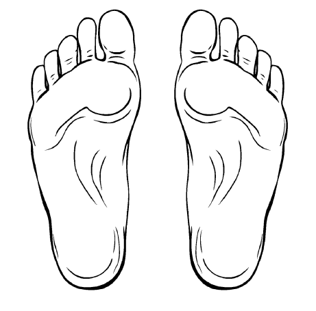
The objective of our algorithm is to classify each subject’s walk into one of the two categories: Parkinson and control. Each recorded walk was documented with 18 VGRF 1D signals, measured in Newtons as a function of time, from several foot sensors. These signals correspond to 8 sensors placed underneath each foot (figure 1), in addition to two more signals that represent the sum of the 8 VGRFs for each foot. The VGRF signals comprise relevant information for gait analysis and characterization. In fact, important clinical spatio-temporal gait features, such as swing phase, stance phase and stride

8

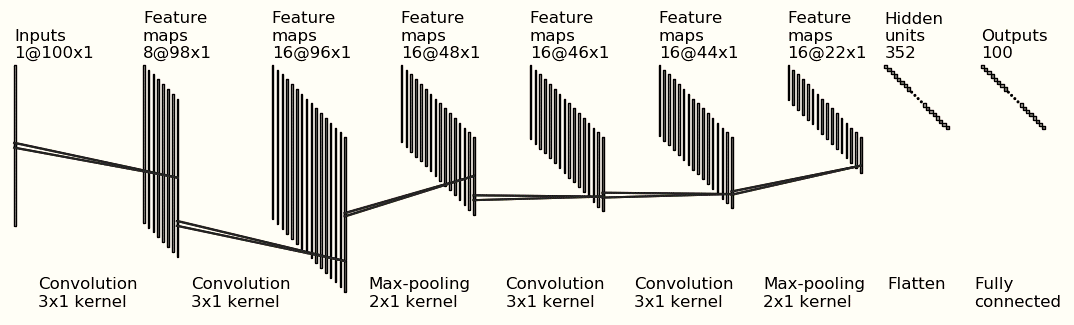
Figure 2: 1D-Convnet: Each 1D-Convnet block is composed of 4 convolutional layers, 2 max-pooling layers and 1 fully-connected layer. time, can be derived from VGRF signals. Feeding our deep learning model with raw data representing vertical ground reaction force records will allow to go beyond the hand-crafted features, by implicitly extracting relevant features for the studied application.

We divided VGRF signals into m segments labeled with the subject cat- egory. These segments are the input samples of our DNN. The DNN is composed of two parts (figure 1). The first part consists of 18 parallel 1D- Convnets, while the second part is a fully connected network that operates on the concatenation of the features extracted by the 18 1D-CNN. The final walk classification was decided according to the majority classification of all the subject segments.

3.2. Parallel 1D-Convnet Branches

The first part of the network is composed of 18 parallel 1D-Convnets (figure 2). Each network takes as input a VGRF signal going through 4 convolutional layers, that lead to a fully connected layer. Every two convo- lutional layers is followed by a max-pooling layer. Each filter in the convo-

9

lutional layers extracts a specific pattern that allows differentiating between the Parkinson and control group. This 1D-Convnets parallelization allows the treatment of each signal independently. In fact, since each sensor records a specific data from a specific point, each time series has its own deep features and is analyzed separately with the 1D-Convnets parallelization.

3.3. Fully Connected Bloc

The second part of the network is designed to learn the relationship be- tween the spatial feature extracted from the 1D-Convnets and the final out- put classification. First, the outputs of those 18 parallel 1D-Convnets are all concatenated into one single vector. This deep feature vector passes through two fully connected layers leading to the output layer. For the Parkinson’s detection, the output layer is composed of one neuron that predicts the classi- fication probability. For the severity prediction, the output layer is composed of 5 neurons (for 5 classes) to predict the final classification. This design has

Two Main Advantages:

• Selection: the network selects the most significant time series that con- tribute the most to the performance of the algorithm. • Abstraction: time series from different sensors are merged together only after passing through the 1D-Convnets. This allows getting significant features at the concatenation step. In fact, at this hidden state, each feature vector is obtained after multiple convolution steps. Therefore it would contain more abstract/global features. In our case, we believe that merging global features together is more efficient than merging

10

raw data at the input level, since it is more robust to noise and local changes.

4.1. Database

We used the public database collected by Physionet 2, which includes data reported by Frenkel-Toledo et al. (2005a,b), Yogev et al. (2005) and Hausdorffet al. (2007). In total, 93 parkinsonian patients and 73 control subjects participated in those studies. Each subject walked on a flat floor for two minutes at their natural pace. For each subject, eight sensors were placed under each foot (figure 1). Each sensor measures the VGRF (in New- ton) under its specific point. The sampling frequency was 100 samples per second. The dataset also includes double-task time series, where subjects were walking while doing another activity. This results in an unbalanced 305 walks recorded (70% Parkinson and 30% control walks). For each walk, 18 time series signals are available: 16 (8×2) VGRF recorded from 8 sensors on each foot and 2 total VGRFs under each foot. For each subject (Parkinson or control), the UPDRS total score is reported in the database. The scores are distributed in a range between 0 and 70.

4.2. Parkinson’S Severity Prediction

We have also tested our algorithm to predict the severity of the Parkin- son’s disease. We used the Unified Parkinson’s Disease Rating Scale (UP-

11

DRS), which is the most used scale for Parkinson severity rating scale (Ra- maker et al., 2002). We segmented the continous scale into 5 levels :

• Class 5: 35 ≤Updrs

We kept the same architecture of the DNN and the same training hyper- parameters. We only modified the last layer. We replaced it with a fully connected of 5 neurons, with a softmax activation layer.

4.3. Evaluation Metrics

We used cross-validation with 10 folds to test our algorithm on 300 walks. We divided each of the Parkinson and the control group into 10 folds at the subject-level. This allowed us to keep the same dataset balance (70 % Parkinson - 30% Control) for each fold. We report the evaluation metrics over the combined validation predictions.

4.3.1. Parkinson and control subject classification The control group is identified as the negative (N) group and the Parkin- son group is the positive (P) group. We use the following notations: • Number of true positive (TP): Parkinson subject correctly classified • Number of true negative (TN): control subject correctly classified

12

• Number of false positive (FP): control subject misclassified • Number of false negative (FN): Parkinson subject misclassified The specificity (Sp), sensitivity (Se), and accuracy (Acc) are calculated

4.3.2. Parkinson Severity Prediction

Since this is a multiclassification experiment, we report the precision, the recall, and F1 score for each class. For each class, true positives (TP) are the patients with the corresponding label who are correctly classified.

4.4. Training

Since deep learning algorithms require large datasets, each walk was di- vided into smaller segments of 100 time steps with 50% overlap. Each seg- ment was labeled with the subject category for the training. This segmen- tation was done inside each fold. Thus, the segments of a given subject are

Related Journal Articles & DOI Links

Selected peer-reviewed publications relevant to 12 Lead ECG Acquisition. Click the DOI to access the full paper (may require institutional access).

Why Choose Us?

Bangalore guidance for robotics, Spectre and autonomous systems projects.