Home Health Monitoring Device

Sage

Wei Liu1,2, Zhilu Lai2,3,4,5, Kiran Bacsa2,3 and Eleni Chatzi2,3

Abstract

Accurate structural response prediction forms a main driver for structural health monitoring and control applications. This often requires the proposed model to adequately capture the underlying dynamics of complex structural systems. In this work, we utilize a learnable Extended Kalman Filter (EKF), named the Neural Extended Kalman Filter (Neural EKF) throughout this paper, for learning the latent evolution dynamics of complex physical systems. The Neural EKF is a generalized version of the conventional EKF, where the modeling of process dynamics and sensory observations can be parameterized by neural networks, therefore learned by end-to-end training. The method is implemented under the variational inference framework with the EKF conducting inference from sensing measurements. Typically, conventional variational inference models are parameterized by neural networks independent of the latent dynamics models. This characteristic makes the inference and reconstruction accuracy weakly based on the dynamics models and renders the associated training inadequate. In this work, we show that the structure imposed by the Neural EKF is beneficial to the learning process. We demonstrate the efficacy of the framework on both simulated and real-world structural monitoring datasets, with the results indicating significant predictive capabilities of the proposed scheme.

Keywords

Neural Extended Kalman Filters, variational inference, learnable filters, deep learning, structural dynamics, structural

Introduction

Digital twins have attracted interest in a wide range of applications, among which structural digital twins have shown promise in virtual health monitoring, decision- making and predictive maintenance1. A digital twin is a virtual representation of a connected physical asset and encompasses its entire product lifecycle2. They acquire and assimilate observational data from the physical system and adopt this information to update dynamics models,

Physical

system3.

The

underlying dynamic model thus significantly underpins the establishment of a digital twin4. Unlike physics-based modeling, which relies on first principles5, data-driven modeling resorts to use of learning algorithms to infer the underlying mechanisms that drive a system’s response6.

The latter class of models plays an essential role in vibration-based structural health monitoring (SHM)7, as a main approach to understanding the actual properties of the assessed structural systems, and to performing accurate dynamical response prediction with the established models.

Diverse data-driven techniques have been developed in the context of SHM, including vibration-based modeling based on modal parameters derived from measured structural response signals8 and conventional time series analysis techniques, including those of the AutoRegressive class9,10.

These methods are typically non-trivial to apply on complex structures with large inherent uncertainties, such as large- scale civil infrastructure systems.

Which

draw from system identification, machine learning (ML) and deep learning (DL), in particular, offer powerful and promising tools for modeling complex systems or capturing latent phenomena. Important applications include image recognition11–13, speech recognition14, autonomous driving15, and more. Their aptitude in recognizing patterns in data and doing so via use of reduced latent features renders such schemes potent tools for large complex structural dynamics modeling7,16,17, which exhibit complex, oftentimes nonlinear, behaviour.

Many Recent Works Have Been Focusing On Bridging

deep learning and structural dynamics18,19. We classify these methods into two main categories, namely direct mappings and generative models. The first class essentially learns a function that maps the input (force/load) to the output (response) of the system. This class of methods

Of

Civil, Environmental and Geomatic Engineering, ETH Z¨urich, Z¨urich,

Switzerland

3Future Resilient Systems, Singapore-ETH Centre, Singapore 138602,

Singapore

4Internet of Things Thrust, Information Hub, HKUST(GZ), Guangzhou,

Corresponding Author:

Zhilu Lai, Internet of Things Thrust, Information Hub, HKUST(GZ), Guangzhou 511458, China. Formerly at Singapore-ETH Centre. Prepared using sagej.cls [Version: 2017/01/17 v1.20]

Journal Title Xx(X)

exploits neural networks with customized architectures

At

hand20–23, such as recurrent neural networks (RNN) and convolutional neural networks (CNN). The caveat of these methods lies in constructing a mere input-output mapping without explicitly modeling the governing dynamics, thus implying that interpretability and generalizability may not be guaranteed. Meanwhile, vibration data measured from operating engineered systems usually embody and reflect the underlying governing dynamics of that system. In this respect, the second class of methods, which fall in the generative model class, attempts to learn a dynamical model that best captures the underlying dynamic evolution. Deep learning-based state space modeling, either in continuous or in discretized format, has been employed to perform data- driven modeling with various deep learning methods24–30.

This class of methods aligns with the common approach to modeling dynamics, rendering such a representation interpretable, even though it is delivered via learned neural network functions. This paper will be focusing on the second class.

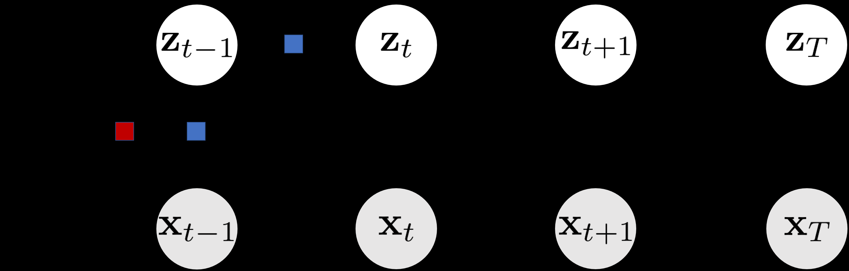
Figure 1. Learning a dynamical system from data using a DL-based state space approach.

As Shown In Figure 1, The Key Idea Of This Second

class lies in learning three models: (i) the inference model: modeling how the latent variable vector z can be estimated from observation/data x; (ii) the transition model: modeling how the latent variable z evolves over time; and (iii) the observation model: modeling how the measured data x are generated from z. For convenience, the transition and observation models are collectively referred to as dynamics models throughout this paper.

Dynamical variational autoencoders (VAEs)29,31 is a class of methods following the architecture described in Figure 1, for modeling a dynamical system from data (x →z →x).

In addition to the dynamics models, the inference models in VAE-based methods are typically parameterized by neural networks. As shown in27,32 and studied further in33, in this setting, the variational objective depends mainly on the inference model, while the dynamic models are relegated to a regularizer for the inference network. Often, this makes the learned model unsuitable for prediction due to the inaccuracy of the dynamics models employed to generate predictions.

On the other hand, while VAEs can be too flexible with both dynamics models and inference models parameterized by neural networks, the conventional Bayesian filtering methods34–36 go to the other extreme, requiring known dynamics models, usually derived from physics-based representations, and conduct the inference only using these dynamics models with no further inference models.

Formulating suitable transition and observation models can be infeasible and challenging in many scenarios, especially when the dynamics of the system is not easily modeled or fully understood, or the sensory observations stem from vision-based data (images, videos). Over the past years, deep learning has become the method of choice for processing such data. Recent work33,37–40 showed that it is also possible to render the dynamics models of Bayesian filters learnable and train them end-to-end, leveraging deep learning techniques and filtering algorithms. For Kalman Filters37, Extended Kalman Filters33, Unscented Kalman Filters38 and Particle Filters39,40, the respective works showed that such learnable filters systematically outperform unstructured neural networks like RNN, LSTM and CNN38.

Combining the benefits of the VAE- and Kalman filtering- based strategies, and inspired by related work in the robotics community33,37–40, we utilize the learnable EKF proposed in33 and name it as Neural Extended Kalman Filter (Neural EKF) in this paper for learning and predicting complex structural dynamics in real scenarios, based on these main principles: (i) we use EKF formulas to conduct closed-form inference instead of implementing an additional neural network to overtake this task, thus allowing for the training to focus on the dynamics models rather than the inference task; and (ii) we eliminate the requirement of explicitly known transition and observation models imposed by conventional Bayesian filtering approaches. At this point, we wish to clarify that the idea we here present is originally adapted from33, where a Replay Overshooting framework is presented. The Neural EKF presented in this paper is a modified version of the previous scheme, adapted to structural dynamics problems. We further wish to clarify that an existing framework termed Neural EKF41 appears in existing literature, which is however different to what we here propose. In that work, the transition model comprises the Jacobian of estimated system dynamics as a prior, with an error correction term modeled by neural networks. That framework is termed Neural EKF due to the use of the Jacobian in the transition model, while the neural network simply learns a discrepancy term. There is no actual extended Kalman filtering process, while further the observation and inference models are not considered, as carried out in this work. Here we choose to term this framework the Neural EKF since our suggested scheme comprises a fully learnable version of the original EKF.

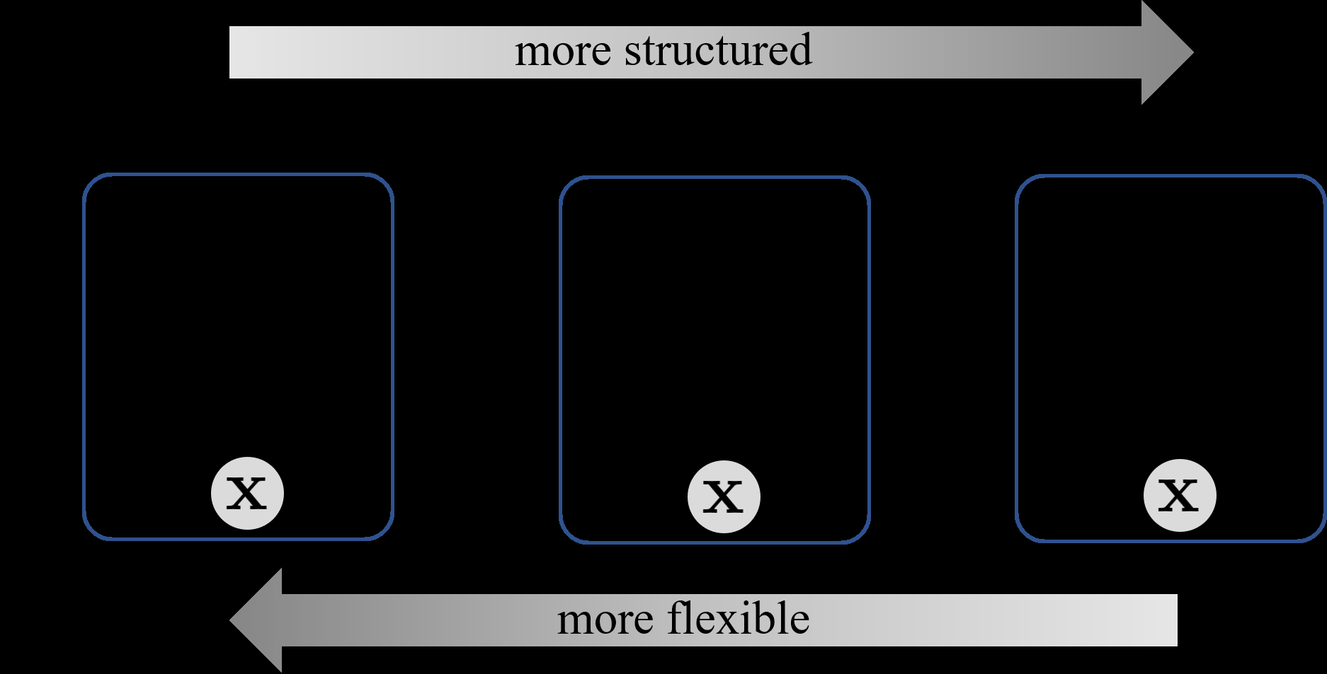
From the perspective of Kalman filtering, the Neural EKF is a learnable implementation of the EKF, where the transition and observation models can be learned by end- to-end training. From the perspective of VAE modeling, the Neural EKF draws from a variational learning methodology with the EKF serving as the inference model, which conducts inference using only dynamics models and does not impose additional hyper-parameters to be learned. We use Figure 2 to summarize the comparisons between VAEs, the Neural EKF and the EKF. We validate the framework on three different scenarios to demonstrate its value in learning dynamical systems. Further to verification on simulated data, two experimental case studies on seismic and wind turbine monitoring are presented to validate the capability of the framework to capture the underlying dynamics of complex physical systems. The scheme is shown to perform accurate predictions, which is essential for adoption in downward applications, such as structural health monitoring and decision making.

Prepared Using Sagej.Cls

Liu et al.

3

Figure 2. Comparison of the variational autoencoder, Neural EKF, and EKF, using a single node as an instance. Solid lines denote the dynamics model. In the VAE and the Neural EKF, the transition model pθt(z) and observation model pθo(x|z), are parameterized by neural networks with parameters θ = θt

S Θo;

dashed lines denote the inference model. Variational autoencoder: the inference network qϕ(z|x) is configured using a separate set of parameters ϕ than the generative model parameters θ. Throughout this paper, the Deep Markov Model (DMM) is adopted as the standard dynamical VAE. Neural EKF: there are no additional parameters ϕ involved for the inference model. Instead, as inference is performed via the linearized Kalman filter equations, the inference model implicitly uses θ that parameterizes the dynamics model. The training process exclusively relies on the parameters θ, thus resulting in a more accurate dynamics model. EKF: there are no learnable parameters involved, and all the governing equations are known, as dictated by the structure of conventional Extended Kalman Filters.

Models

Variational autoencoders (VAEs)31 are popularly used for capturing useful latent representations z from data x by reconstructing the VAE input to an output vector. The VAE can be extended to a dynamical version by considering the temporal evolution of the latent variables29. Among various dynamical VAEs, Deep Markov Models (DMMs32) offer a primary example of unsupervised training of a deep state-space model. By chaining an approximate inference model with a generative model and using the variational lower bound maximization approach, DMMs deliver the most direct extension of static VAEs to account for temporal data29. The DMM couples a transition model pθ(zt|zt−1), describing temporal evolution of the latent states, with an observation model pθ(zt|xt), serving as a decoder and describing the process from latent states to observations, and an inference model qϕ(zt|x1:T ), serving as an encoder, which approximates the true posterior distribution p(zt|x1:T ).

The training of a VAE consists in maximizing a variational lower bound of the data log-likelihood log p(x). Upon application of the variational principle on the inference model qϕ(zt|x1:T ), the evidence lower bound (ELBO) of the

(1)

where the KL-divergence is defined as KL[q(z)||p(z)] :=

P(Z)Dz. Apart From The Parameters Θ Involved

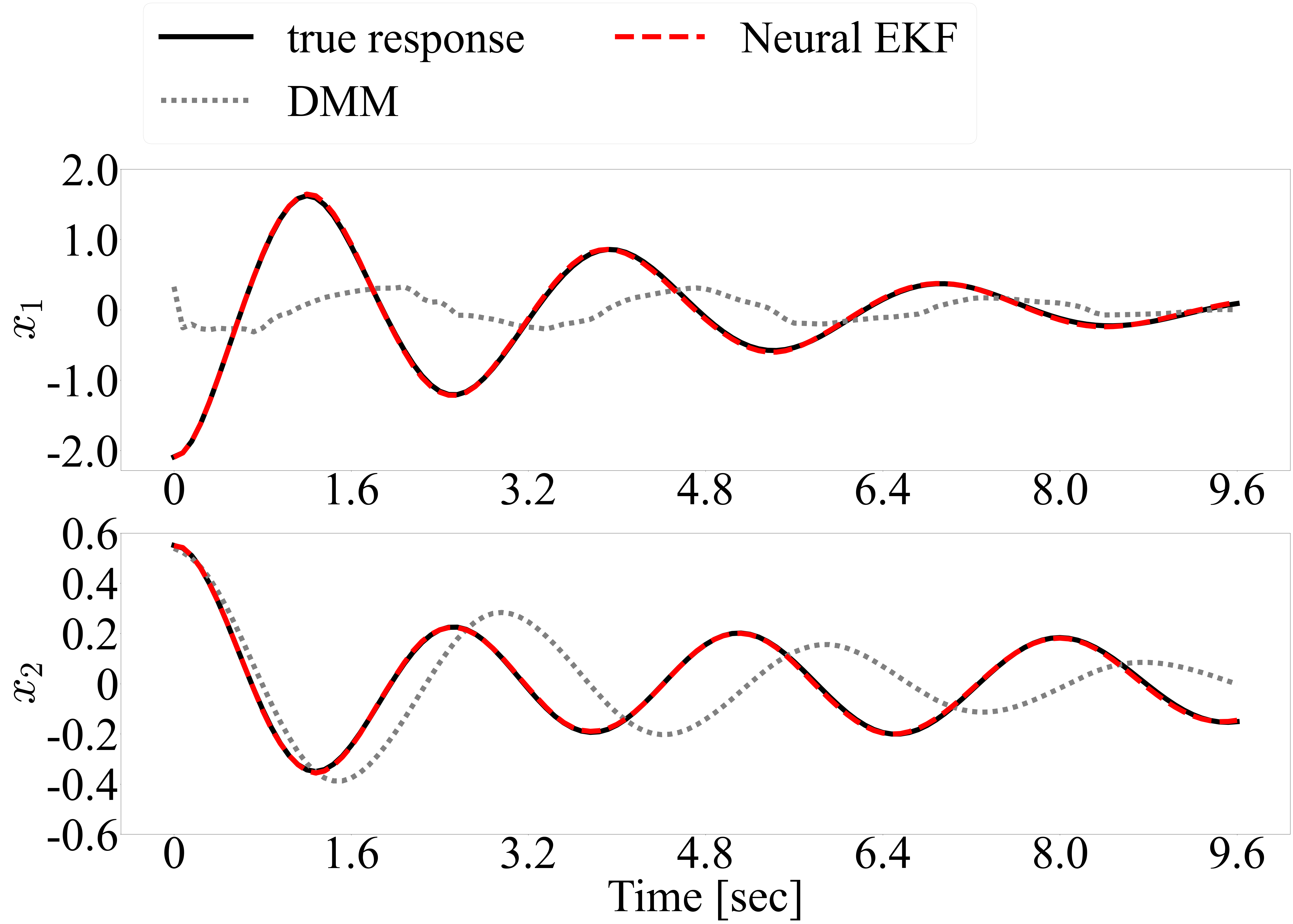
Figure 3. Comparison of predictive capabilities of the DMM versus a Neural EKF on a 2-DOF Duffing oscillator system. The

Displacement Response Is Assumed To Serve As The

measurements set. in transition and observation models, the VAE architecture typically employs an additional inference network, which is independently parameterized by the hyper-parameters ϕ of the corresponding neural networks. The key idea of VAE is to approximate the posterior distribution with the introduced inference network. However, the objective function ELBO largely depends on the quality of the inference model through the first reconstruction term, which does not involve a transition model, and the influence of the transition models is indirectly relegated to a regularizer for the inference model, reflected in the second KL-divergence term33. The KL-divergence itself is a regularization term and it attempts to only make the single-step dynamics transition similar to the posterior given by the inference network. The above arguments indicate that the quality of VAE reconstructions, as measured by the value of the objective ELBO, strongly depends on the inference model but rather weakly on the transition models. This characteristic of the training objective makes the learned model capable of delivering accurate inference results under availability of observation (monitoring) data, but unsuitable for prediction due to the insufficient training of the transition models.

As shown in Fig. 3, the result demonstrates the advantages of the Neural EKF over the DMM, which is, as mentioned, a dynamical VAE model that directly extends the static VAE to account for temporal data. The results are demonstrated on a 2-DOF Duffing system, defined by Equation (28) appearing in the Applications section. It is observed that the DMM fails to deliver sufficiently accurate predictions, while the predicted responses, furnished by the Neural EKF, very well fit the true (reference) responses.

Extended Kalman Filtering And Smoothing

For nonlinear state estimation and parameter identification in civil and mechanical engineering, the Extended Kalman

Filter (Ekf) Has Been A Popular Choice For Weakly

nonlinear systems, mainly due to its ease of implementation, robustness and suitability for real-time applications. It

Journal Title Xx(X)

assumes a sequence of measurements x1:T from a monitored dynamical system, which are generated by some latent states z1:T that are not necessarily directly observed. The transition from a state zt−1 to the next state zt is termed as transition, and the process from a state zt1 to its corresponding observation xt is termed as observation. Compared to dynamical VAEs, the EKF assumes that the transition and observation models are given, as described by the following

(3)

where f and g are two known linear/nonlinear functions governing the transition and observation models, and wt ∼ N(0, Qt), vt ∼N(0, Rt) are Gaussian noise sources with mean zero and covariances Qt and Rt, respectively. EKF assumes that the inferred posterior distributions of latent states are based on past and current observations x1:t and driving force u1:t, and follow a Gaussian distribution:

(4)

Here µt|t and Σt|t represent the mean and covariance of the posterior distribution. The Kalman Filter (KF)42 offers a closed-form of the posterior distributions q(zt|x1:t, u1:t) of latent states and provides exact inference for linear systems.

The EKF conducts approximate inference, employing a linearization of the nonlinear equations. For EKF, the inference of the posterior distribution is obtained by iteratively executing the following two steps. The first step predict is to compute the posterior distribution q(zt|x1:t−1, u1:t−1) = N(µt|t−1, Σt|t−1), which is simply

Is The Jacobian Of F At

µt−1|t−1. The second step update pertains in updating the posterior distribution from the predict step using the current

∂Μt|T−1

is the Jacobian of g at µt|t−1. The Jacobian matrices At and Ct are used as linear approximations of the original nonlinear functions f and g, respectively, for conveniently computing the involved covariances Σt|t−1 and Σt|t.

The EKF is a recursive filtering method for conducting inference based on x1:t, i.e., the observations until the present time t. Since we assume that a sequence of observations x1:T is available, it is possible and reasonable to further update the inference of posterior distributions with the whole sequence of observations, with respect to a time step within the sequence. This process is termed as smoothing. The Rauch-Tung-Striebel smoothing43 is a Kalman smoothing algorithm to infer such posterior distributions q(zt|x1:T , u1:T ) = N(µt|T , Σt|T ) of latent states based on the whole sequence of available observations.

The smoothing process can fully make use of available data when computing the posterior distributions and generate more accurate inference results with adequate information, instead of only utilizing information before each time step, which is the case for the Kalman filtering process. Note that, compared to Eq.(4), now the posterior depends on the whole sequence of x1:T and u1:T . Once the EKF process is completed, the smoothing algorithm operates in a backward manner, from time T to 1, to update the posteriors:

T(Σt+1|T −Σt+1|T)(Ks

t)T .

(12)

The intermediate quantities µt|t, µt+1|t, Σt|t and Σt+1|t in this smoothing process are already available at Eqs.(5)-(9), in the EKF stage.

Prior And Posterior Distributions

Here we introduce the prior and posterior distributions that will be used for computing the loss function of Neural EKFs in the later section. The final posterior distribution after application of the EKF algorithm and the smoothing step is given as q(zt|x1:T , u1:T ) = N(µt|T , Σt|T ), where µt|T and Σt|T are given in Eqs.(11) and (12). Furthermore, given zt−1 ∼N(µt−1|T , Σt−1|T ), we can compute the

Is The Jacobin Of F

at µt−1|T . Subsequently, the distribution of observation p(xt|zt), given zt ∼N(µt|T , Σt|T ), can be derived as

∂Μt|T

.

Neural Extended Kalman Filters

A salient limitation of the EKF when applied to learning dynamical systems lies in the requirement for the transition model f and the observation model g to be explicitly defined or at least of known functional format. However, this is not practically feasible when applied to real-world complex systems. In tackling this limitation, the key idea of the proposed Neural EKF is to replace f and g by learnable functions, typically by neural networks. By doing this, the transition and observation models turn to be trainable and efficiently learned by minimizing the defined loss function, making the Neural EKF a flexible tool for learning the dynamics of complex systems. Also, another benefit compared to VAEs, where the inference model is parameterized by neural networks, is that the inference model of the Neural EKF follows a closed-form model. In this section, we will detail the modeling and training of the Neural EKF framework.

Prepared Using Sagej.Cls

Liu et al.

Dynamics Models

In Eqs.(2) and (3), if we replace f and g by learnable transition and observation functions, the framework can be

(16)

where fθt and gθo are the learnable functions governing the transition and observation models, both parameterized by

S Θo. The Process

noise sources wt and observation noise vt are assumed to follow Gaussian distributions, with respective time-invariant covariances, i.e., wt ∼N(0, Q) and vt ∼N(0, R) for all time steps t. The time-invariant covariances Q and R are also set as learnable parameters during the training process. It is noted that here the latent dynamics is formulated as a discrete model. Alternatively, continuous models such as Neural Ordinary Differential Equations18 can also be implemented to model the latent dynamics if one wants to treat the latent dynamics as a continuous model, as explained in Appendix.

The Inference Model Of The Neural Ekf Follows The

format of the EKF. This is different from the inference model in VAEs, where qϕ is a separate inference network parameterized by ϕ independent of parameters within fθt and gθo. Since the objective ELBO largely depends on the goodness of reconstruction and inference, a separate inference network is thus weakening the training of the transition and observation models.

Evidence Lower Bound And Training

With Kalman filters conducting inference, the parameters to be learned are summarized in the vector θ, which includes neural network parameters of both the transition model fθt and the observation model gθo. In addition, the initial values µ0|0 and Σ0|0 and covariances Q, R for respective noises are also parameters to be learned. Similar to the VAE, the training of Neural EKFs is embedded in the variational inference methodology, with the EKF algorithm charged with conducting inference. Given any inference model qϕ(zt|x) and Markovian property implied by the dynamics, the ELBO in Eq.(1) can be expressed in a factorized form (x1:T and u1:T are abbreviated as x and u in the following

Actually

qθ(zt|x, u), which alleviates the requirement of additional parameters, further to θ, within the transition and observation models, and thus L(θ, ϕ; x) reduces to L(θ; x). Since the posterior distributions qθ(zt|x, u) can be computed in closed form by EKF, the distributions in Eq.(17) can thus be computed explicitly given zt ∼N(µt|T , Σt|T ), as shown in Section Prior and posterior distributions. Thus, the ELBO

,

given zt ∼qθ(zt|x, u).

(18)

The above involved distributions are based on the prior zt ∼ N(µt|T , Σt|T ). The log-probability and KL-divergence can be computed analytically when all the involved distributions are Gaussian. The log-probability of a Gaussian distribution

(19)

where dx is the dimension of x. As stated in Eq.(14), since zt ∼qθ(zt|x, u) = N(µt|T , Σt|T ) and replace g by gθo, we

T|T + R) . Using

Eq.(19), the log-likelihood term log pθo(xt|zt) in Eq.(18) can

(20)

Similarly, the KL-divergence term KL(q(z)||p(z)), when p(z) = N(µp, Σp) and q(z) = N(µq, Σq) are both Gaus- sian distributions, comprises an analytical form as:

(21)

where dz is the dimension of z. As stated in Eq.(13), and

T−1|T + Q) (22)

since we have zt−1 ∼qθ(zt−1|x, u) = N(µt−1|T , Σt−1|T ) and zt ∼qθ(zt|x, u) = N(µt|T , Σt|T ). Substitute these mean and covariance into Eq.(21), the KL-divergence term

I

.

(24)

Typically, the variational objective function for the dynamical VAE framework focuses on the reconstruction loss, which largely depends on the inference model (encoder) and observation model (decoder), whereas the transition model plays a minor role in the variational objective and works as an intermediate process for training. This often results in an accurate inference model and a less meaningful transition model, which is not applicable for prediction because the transition model cannot reflect the true underlying dynamics. Therefore, it is necessary that the objective function also takes the accuracy of the transition model into consideration to ensure its closeness to the true latent dynamic process. To address this issue, we adopt the overshooting method proposed in33, which is termed as replay overshooting. The key point lies in simply introducing the prediction loss of the generative model into the objective function. After obtaining a sequence of means and covariances {(µt|T , Σt|T )}, the initial value (¯µ0, ¯Σ0) = (µ0|T , Σ0|T ) will be further used for prediction process.

Then similarly as the prediction step in EKF, the predicted

¯Q(Zt) =

N(¯µt, ¯Σt) from the generative model. The final reconstruc- tion loss is composed of the both sets of posterior distri- butions, i.e., the posterior distributions obtained from the Kalman inference model in Eq.(20), as well as those obtained from the transition model, weighted by α (in this paper, we set α = 0.5). These form the objective function combined

(27)

where the first and third term are the same as in (24), while the second term is for overshooting.

The Pipeline Of The Neural Ekf Is Summarized In

Algorithm 1.

Neural Ekf For Response Predictions

Once a Neural EKF model is trained, the learned function fθt and gθo is available and can be used for response prediction. The prediction is performed using zt = fθt(zt−1, ut−1) and xt = gθo(zt), given a new initial condition z0 and corresponding driving forces u1:T . Note that a new initial condition can be either specified by the user, or inferred from actual data via use of the inference model of the Neural EKF.

The Neural EKF is capable of generating predictions in real-time to detect structural anomalies and changes as they occur for structural health monitoring. On the other hand, it requires offline training on a characteristic batch of operational data, prior to it being applied in prediction mode.

However, in intervals where loads significantly increase with respect to the training set, possibly triggering more severe nonlinearity, or if the system experiences damage, the model must be updated offline using newly acquired data for training, in order to adapt to the changed dynamics. This is a trade-off that is often present in real-time monitoring systems, where the need for accurate predictions must be balanced with the need for timely updates.

Application Case Studies

We verify and validate the proposed Neural EKF framework on both simulated and real-world datasets. The numerical simulation aims to demonstrate the predictive capabilities of the learned model via Neural EKF, as compared against the commonly adopted option of variational autoencoders.

The experiments involving real-world monitoring datasets aim to further demonstrate the Neural EKF’s ability to learn the dynamics when the system is considerably complex.

In this case, physics-based modeling can be challenging due to the unknown model structure, or computationally unaffordable. In the employed seismic monitoring case study, we validate the effectiveness of the Neural EKF in predicting seismic responses on the basis of available ground motion inputs (earthquakes). Furthermore, in the experimentally tested wind turbine case study, we perform a thorough analysis on dynamic response prediction, damage detection and structural health monitoring based on the learned Neural EKF model.

The transition function fθt and observation functions gθo are modeled as multilayer perceptrons consisting of three

Prepared Using Sagej.Cls

Liu et al.

7

hidden layers. Each hidden layer comprises 64 nodes for the Duffing and seismic response examples, and 128 nodes for the wind turbine example. The dimension of the latent states zt is assumed to correspond to twice the DOFs of the modeled system, which is an assumption commonly adopted in conventional state-space modeling. The dimension of latent states is a predefined hyperparameter and can be fine- tuned if needed. This is different from conventional Kalman filters, where a fixed state equation, and thus a corresponding dimension, has to be assumed. In this case, issues may arise in terms of the observability of the system’s states, in case the observed variables are not carefully chosen, and particularly if they are lower than the number of predefined latent states. However, in our proposed method, the latent state mainly serves as an intermediate quantity to optimally reconstruct and predict the observed quantities. Similar to the width and depth of neural networks, a larger latent state dimension usually benefits the training result but may lead to overfitting. In our examples, we opted for a latent state dimension that equals twice the number of DOFs of the modeled system, as this is a natural choice. The data and codes used in this paper are publicly available on GitHub at https://github.com/liouvill/NeuralEKF.

Duffing Oscillator System

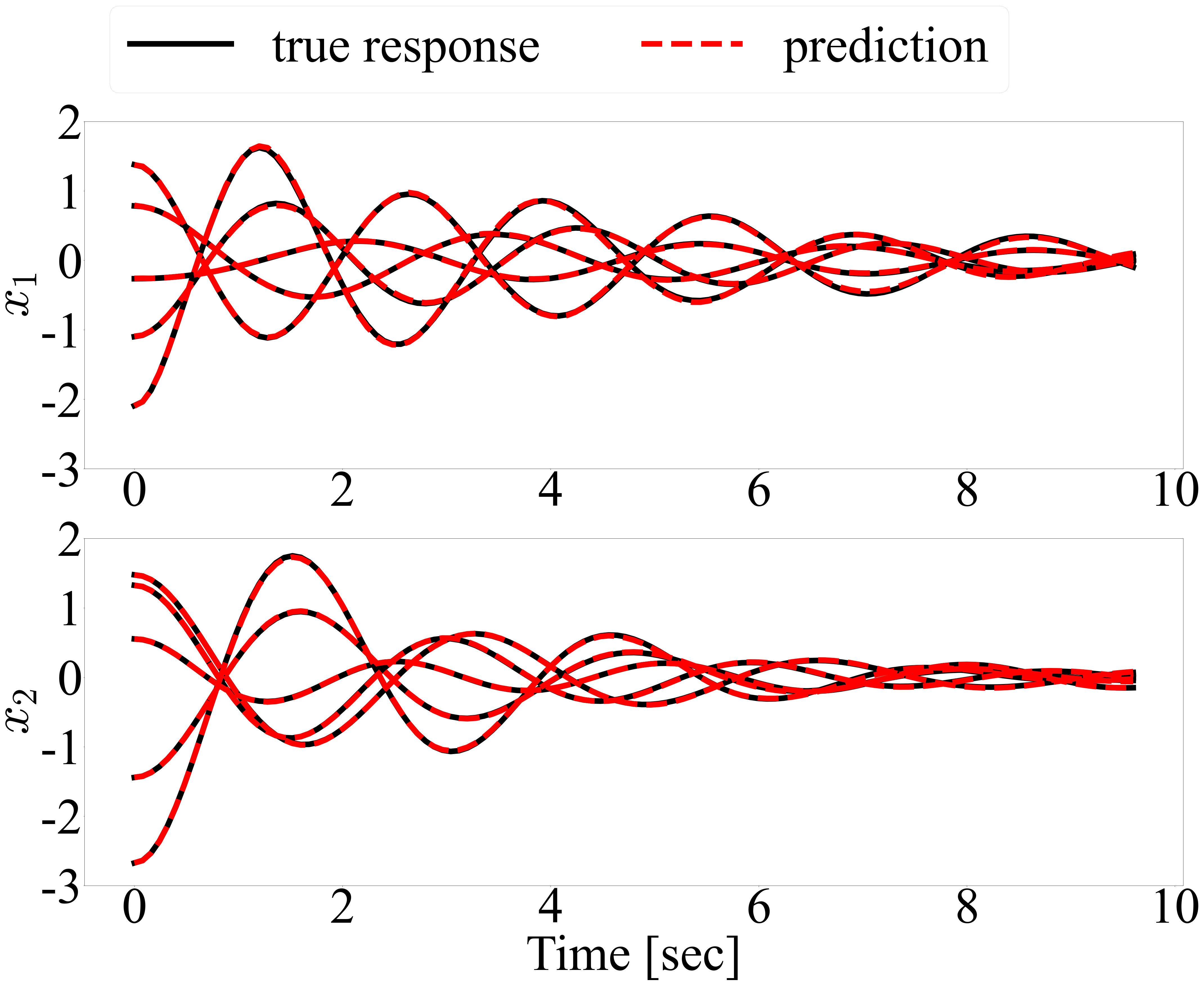
Figure 4. Predicted results for the simulated 2DOF Duffing system. We first demonstrate the performance of the Neural EKF framework for predicting the dynamic response through a numerical example. In this example, we consider a 2 degrees- of-freedom (DOF) nonlinear duffing oscillator subjected to random excitations. The data used for this case study are

And The Coefficient Of The Cubic Stiffness Term

kn = 1. Here the displacements of both DOFs x1 and x2 are assumed available as measurements. It is noted that this parameter setting falls into the scenario where the Duffing oscillator presents a single stable equilibrium point at the origin. We consciously make this choice, as we here adopt this as a nonlinear example, in order to demonstrate the capability of the Neural EKF to deal with nonlinearity, but not rare instabilities or chaotic behavior, which would require a more complex treatment.

For This Numerical Case Study, A Number Of 1000

random trajectories are generated with both transition and observation noise variances equal to 0.001 for training by the simulated 2-DOF nonlinear Duffing system shown in Eq.(28). Another 5 randomly generated trajectories are used as an unknown dataset for testing the prediction capability of the Neural EKF framework. The prediction results for the free vibration case are shown in Figure 4. As indicated by the results, the Neural EKF is capable of producing satisfactory predictions that reasonably match the reference well for this simulated nonlinear system. As comparison, which is already shown in Fig 3, it is observed that the DMM, which is a pure VAE-based method, fails to capture the dynamics and the predictions are much less accurate.

0.01709

Table 1. Comparison with noise-free system responses under different noise levels: RMSE1 is for x1 and RMSE2 is for x2. To further demonstrate the robustness of the proposed model, we have generated artificial observations (measured data) with different levels of noise contamination. The data is generated by Eq.(28) using the same initial values across three cases, but with different levels of additive Gaussian observation noise. More specifically, we generate three different simulated cases corresponding to an observation noise variance of 0.001, 0.01 and 0.1, respectively. The “process noise” is set to be zero, when generating artificial observation data, since integration of a larger transition process noise would cause the solution of the ODE to diverge due to nonlinearity of the Duffing system. The root mean squared error between the predicted and true (noise- free) system response is reported in Table 1. Our results indicate that the difference between the predicted and noise- free system response, for training and prediction under assumed contaminated measurements, are similar across different noise covariance levels. The proposed method thus proves particularly robust to noise contamination, as revealed by the results shown in Figure 5 for the case with different observation noise variances. As comparison, the DMM-predicted results are plotted in dark green, which deviate significantly from the ground-truth and fail to provide accurate and reliable predictions.

Related Journal Articles & DOI Links

Selected peer-reviewed publications relevant to 12 Lead ECG Acquisition. Click the DOI to access the full paper (may require institutional access).

Why Choose Us?

Bangalore guidance for robotics, Spectre and autonomous systems projects.