Metered Dose Inhaler Sensor

Graphical Abstract

A computational fluid dynamics model for the simulation of flash- boiling flow inside pressurized metered dose inhalers

Highlights

A computational fluid dynamics model for the simulation of flash- boiling flow inside pressurized metered dose inhalers

Riccardo Rossi, Ciro Cottini, Andrea Benassi

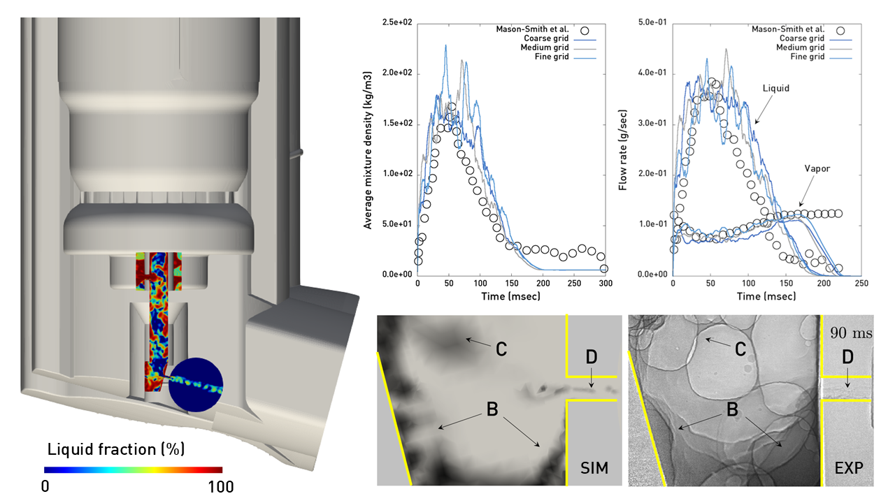
• The CFD model successfully simulates the metered discharge in a pMDI • Good agreement with experiments is found for mixture profiles at noz-

Zle Orifice

• Equilibrium cavitation models are able to represent the flash-boiling

Flow

• Turbulent fluctuations do not impact significantly the metered dis-

Charge

• Effects of geometrical modifications on metered discharge are captured

A Computational Fluid Dynamics Model For The

simulation of flash-boiling flow inside pressurized

Metered Dose Inhalers

Riccardo Rossia,∗, Ciro Cottinib, Andrea Benassib,c

Bchiesi Farmaceutici S.P.A., Parma, Italy

cInternational School for Advanced Studies (SISSA), Trieste, Italy

Abstract

In this work we present, for the first time, a computational fluid dynamics tool for the simulation of the metered discharge in a pressurized metered dose inhaler. The model, based on open-source software, adopts the Volume- Of-Fluid method for the representation of the multiphase flow inside the device and a cavitation model to explicitly account for the onset of flash- boiling upon actuation. Experimental visualizations of the flow inside the device and measurements of the mixture density and liquid and vapor flow rates at the nozzle orifice are employed to validate the model and assess the sensitivity of numerical results to modeling parameters.

The Results

obtained for a standard device geometry show that the model is able to quantitatively predict several aspects of the dynamics and thermodynamics of the metered discharge.

We Conclude By Showing How, By Allowing To

reproduce and understand the fluid dynamics upstream of the atomizing nozzle, our computational tool enables systematic design and optimization of the actuator geometry.

Keywords:

pMDI, therapeutic aerosol, CFD, multiphase flow, internal

∗Corresponding Author

Preprint submitted to Int. J. Pharm.

1. Introduction

The wide adoption of pressurized Metered Dose Inhalers (pMDI) for the administration of orally inhaled drug products stems from their low cost, reasonable delivery efficiency and versatility. In fact, Dry Powder Inhalers (DPIs) have much higher costs, while nebulizers require long administration times, need to be connected to a plug or a battery and usually lead to large drug waste. Being the aerosol generated through a propellant, the delivery performance of pMDIs are less sensitive to the patient inspiratory effort than DPIs. However, pMDIs also come with limitations: first, they require the patient to coordinate its inspiratory act with the triggering of the inhaler and secondly, they make use of propellants and solvents, such as ethanol, and they are thus not adequate to deliver bio-molecules [1, 2, 3, 4].

Many factors influence the pMDIs inhalation performance. The choice of the propellant determines the maximum pressure achieved during actua- tion upstream of the atomizing nozzle, impacting the initial droplet size , whereas the concentration and physico-chemical properties of the solvent de- termine the droplet evaporation time and thus the progressive reduction of the Mass Median Aerodynamic Diameter (MMAD) of the airborne aerosol [6, 7, 8]. Propellant and solvent choice, as well as the solvent concentration in the mixture, affect plume velocity and plume angle, determining how much aerosol is held back in the mouth-throat tract [9, 10].

Design And Opti-

mization of pMDI products could definitely become faster and cheaper if these aerosol characteristics could be predicted, using mathematical mod- els and simulations, solely based on the drug product composition and its physico-chemical properties. However, aerosol droplet formation in an atom- izing nozzle is a complex physical phenomenon to study, different types of mechanical instabilities are at play depending on the dimensionless Weber number, i.e. the ratio between the droplet inertial force and its surface ten- sion force. Both experimental imaging and simulation of droplet formation are very demanding tasks, this is why many empirical correlations have been developed to predict the MMAD of the generated droplets based on the noz- zle geometry and the fluid mixture properties. Most used, among them, is

(1)

with pin being the pressure upstream of the nozzle, i.e. in the expansion

2

chamber, pamb the ambient pressure downstream of the nozzle, χ is the vapor quality factor (the mass of vapor divided by the total mass of the mixture in the unit volume) and C is a fitting constant equal to 1.82 in case of a metered discharge. The equation contains no explicit nozzle geometric pa- rameter; however, the pressure drop between the expansion chamber and the ambient pressure depends implicitly on the nozzle diameter and takes different values whether the flow at the nozzle is subsonic, critical (choked) or supersonic. Other simple equations have been developed to estimate the droplet initial velocity and the aerosol production rate [5, 11, 12]. As for the Clark correlation (1), they all depend on dynamics and thermodynamics properties of the mixture upstream of the nozzle. Therefore, the problem of predicting pMDIs delivery performance requires the capability to calculate the aerosol physical characteristics and, in turn, the prediction of mixture properties inside the pMDI during administration. A first attempt in this sense was made in 1975 by Fletcher through a mathematical model of the metered discharge, subsequently extended and improved by many au- thors [11, 14, 15, 16, 17].

System Models Similar To The One Of Fletcher,

where a zero or one-dimensional representation of the pMDI is introduced, allow to predict the temporal evolution of the mixture properties by solving the integral balance equations for the mixture in the main device components.

Several assumptions need to be made in the framework of these models, such as the type of flow regime and the value of discharge coefficients through the orifices. Moreover, system models are unable to study the effect of design changes on the pMDI performance and operation.

Most of the experimental effort is devoted to the characterization of the generated aerosol plume in terms of droplets size and speed, using laser light scattering techniques such as phase Doppler anemometry and particle image velocimetry , or in terms of plume geometry and temperature [20, 21, 22]. Little is known about the flash-boiling of propellant and the fluid dynamics upstream of the atomizing nozzle, i.e.

inside the actuator.

In

this sense a seminal paper is the one by Mason-Smith et al. , where X- ray phase contrast imaging and quantitative radiography have been used to investigate the behavior of the solvent-propellant mixture during actuation, while the liquid and mass flow rate at the nozzle outlet have been quantified optically. The same imaging technique has been adopted more recently by McKiernan to further study the structure and dynamics of the flashing flow in the pMDI, but without providing quantitative information on the mixture during the metered discharge. Temperature profiles during the shot

3

were measured by Gavtash et al. and Myatt et al. in the sump and nozzle-orifice, respectively, whereas Myatt et al. [27, 28] and Gavtash reported measurements for the near-orifice mixture velocity downstream of the nozzle orifice.

In the context of pMDI design, Computational Fluid dynamic (CFD) simulations are usually applied to study the behavior of the aerosol plume downstream of the device [30, 31] and the consequent aerosol deposition in

Patient Mouth-Throat Tract And Bronchial Tree

[32, 33, 9, 34].

Here, For

the first time, we demonstrate the possibility of using a multiphase CFD model to simulate the metered discharge upon actuation, capturing the pro- pellant dynamics in time and in a realistic three-dimensional geometry for the actuator, from the metering chamber to the nozzle orifice. Details on the simulated geometry and pMDI operating conditions are illustrated in Section 2. The computational model is presented in Section 3 along with the physical and numerical assumptions implied in its development.

The

Results section opens with a qualitative description of the metered discharge and its comparison with available experimental imaging data, and continues with the model calibration step, a grid-sensitivity study and by analyzing the effect of including temperature dependence of the physical properties of the mixture as well as the latent heat due to phase-change. A final section illustrates how the simulation tool can be used to predict the effects on the metered discharge from modifications in the actuator geometry and volume.

The Conclusions section summarizes the outcome of the present study, the open points and the need of new measurements to challenge and extend the predictive capabilities of the model.

2. Device Geometry And Operating Conditions

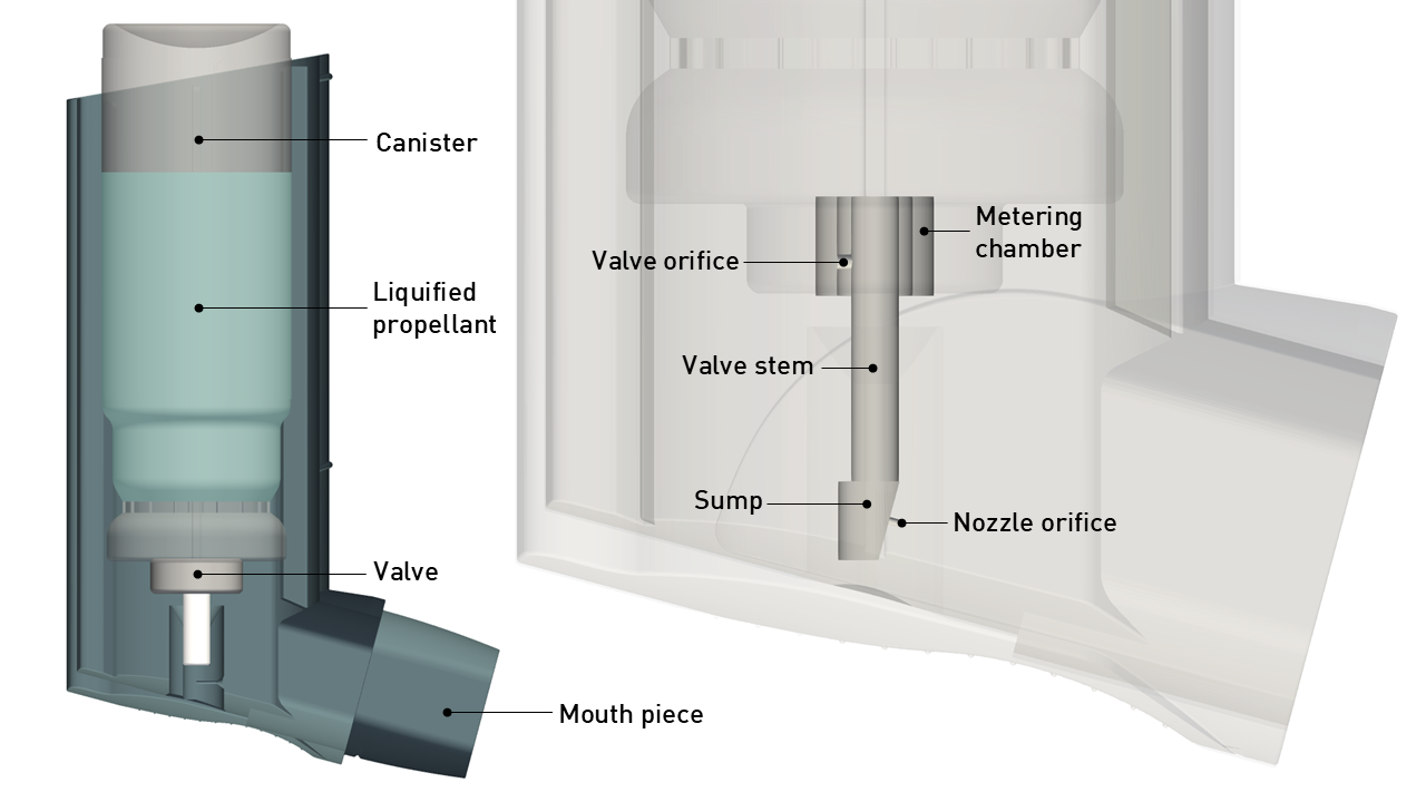
In a pMDI device, shown in Fig. 1, the Active Pharmaceutical Ingredient (API) is solubilized or suspended in a liquid mixture composed by a propel- lant, usually a hydrofluoroalkane (HFA) and by a solvent, typically ethanol.

The mixture is contained inside a metallic canister in equilibrium with its vapor phase, i.e. at its vapor pressure, typically between 3 and 5 bar. A valve is crimped on the canister with a metering chamber whose aim is to collect the dose volume, usually few tens of µL. Upon actuation, the dose is isolated from the canister and exposed to ambient pressure, thereby induc- ing the so-called flash-boiling phenomenon, an extremely rapid and violent phase-change process during which the liquid and vapor mixture is initially

4

Figure 1: Overview of the pressurized metered dose inhaler (left) and main device com- ponents involved in the metered discharge (right). flushed from the metering chamber into the valve stem through the valve ori- fice and subsequently collected into the sump region. From this region, the mixture enters the nozzle orifice undergoing atomization, which ultimately generates the aerosol delivered to the patient through the mouthpiece.

In the present work, the metered discharge of a 50 µL dose of pure HFA- 134a propellant is investigated by numerical simulations. The size of the me- tered valve and the device internal geometry corresponds to the one adopted in the experimental work by Mason-Smith et al. , which will represent the main reference experiment for the validation of the numerical model pre- sented in this study. The valve and nozzle orifice diameters are 0.6 mm and 0.3 mm, respectively, and the valve stem is 12 mm and 2 mm in length and diameter, respectively. The propellant is stored at 5.9 bar, representing the nominal saturation pressure of the HFA134a at room temperature of 20 ◦C.

From the experiments, a typical duration of the metered discharge between 250 ms and 300 ms is observed, which will be replicated in the simulations.

3. Computational Model

The computational model of the pMDI consists of a numerical represen- tation in both space and time of the flow inside the device. Compared to most advanced system models , where only the temporal evolution of the quantities of interest can be predicted, the model is also capable of providing a spatial description of such quantities during the metered discharge. This allows to extend the predictive capabilities of simulation tools to the effect of modifications to the pMDI internal geometry, yet to be explored, on device operation and performance.

The model is developed using the open-source software OpenFOAM® , based on the unstructured finite-volume method, where the flow governing equations are solved on a computational grid consisting of a finite number of cells representing the volume inside the metered-valve, valve stem and sump regions. In the following sections, the governing equations of the multiphase flow model and of the model adopted for the simulation of the flash-boiling phenomenon are presented, along with the computational grid and numerical methods employed to solve the equations.

3.1. Multiphase Flow Model

The flow inside a pMDI is represented by a two-phase (liquid and vapor) mixture originating from the flash-boiling occurring inside the metered valve upon device operation. In the present work, a Homogeneous Fluid Model (HFM) is employed to represent the mixture, where mechanical and thermo- dynamic equilibrium is assumed between the two phases, which thereby share the same pressure, temperature and velocity. Based on these assumptions, a single set of governing equations consisting of the continuity, momentum and energy equations can be solved for the mixture:

6

where ρ, p, Uj and T are the density, pressure, velocity and temperature of the mixture, µ and λ are the molecular viscosity and thermal conductivity and µt and λt are the turbulent viscosity and thermal conductivity associated with the modeling of the turbulent regime of the mixture flow, which will be discussed in Section 3.2. The terms ρgi and fσ in Eq. (3) represent the gravity and surface tension forces, whereas the source terms Sm and ST on the right-hand side of Eqs. (2) and (4) represent the effect of the phase-change due to the flash-boiling of mixture pressure and temperature, which will be introduced in Section 3.3.

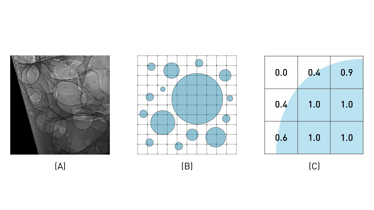
Flow visualizations inside the pMDI performed with X-ray phase con- trast imaging reveal a dispersed regime in the two-phase flow, where numerous bubbles presenting a broad range of scales are present within the propellant undergoing flashing, as shown in Fig. 2(a).

An Explicit Model

of such flow regime, where bubbles with significantly different length-scales must be solved directly, is computationally prohibitive due to the grid resolu- tion needed to capture the liquid-vapor interfaces, as depicted in the cartoon (b) in the same figure. A simplified representation of the two-phase flow based on the Volume-Of-Fluid (VOF) approach is thus adopted here, where the volume-fraction concept is introduced to estimate the amount of liquid and vapor phase present in each computational cell, as shown in Fig. 2(c).

The volume-fractions of the liquid and vapor phases of the mixture are defined as αl = Vl/V and αv = Vv/V , respectively, where Vl and Vv denote the volume occupied by the liquid and the vapor phase inside the volume V of the computational cell. In the present model, an additional transport equation is solved to predict the volume fraction of the liquid phase inside

(5)

where αv is the vapor volume-fraction and where the source term Sαl, which will also be presented in Section 3.3, represents the effect of phase- change associated with the flash-boiling on the liquid volume-fraction. The third term on the left-hand side of Eq. (5) is an artificial compression term used to resolve the interface between the two-phases. Given the dispersed flow regime associated with the pMDI, such term is kept in the present for- mulation for sake of numerical stability, but the liquid-vapor interface cannot be captured accurately because of the limited grid resolution adopted in the calculations, aimed at reducing the computational effort.

7

Figure 2: Volume-fraction based representation of the multiphase flow inside the pMDI: (a) X-ray visualization of bubbly flow in the nozzle region of the device extracted by the original movie (courtesy of Mason-Smith et al. ) (b) sketch of bubbly flow on a finite- volume grid, (c) visualization of the liquid volume fraction in a finite-volume grid.

The properties of the mixture are calculated based on the local volume fraction of liquid and vapor. Due to mass-conservation, the volume fractions of the mixture obey to αl + αv = 1. Therefore, only the transport equation for the liquid volume fraction (5) can be solved and the properties of the

D = Dlαl + Dv (1 −Αl)

The properties of the liquid and vapor phase are obtained from the mea- surements of Tillner-Roth and Baeh , which characterize the propellant over a wide range of temperatures and pressures. In the calculations, the densities of both vapor and liquid are assumed variables to allow for the simulation of the compressible discharge of the propellant from the metered valve. The vapor density is computed via the ideal-gas equation, whereas a reciprocal polynomial function is employed to compute the liquid density based on the pressure and temperature of the mixture:

(7)

where a fit to measured data is performed to compute the coefficients of Eq. (7). Separate calculations are performed considering the remaining properties of both phases, i.e. the dynamic viscosity, specific heat capaci- ties and thermal conductivity, either constant or temperature-dependent to study the effect on the simulated metered discharge. In the case of constant properties, the values measured at room temperature are employed in the computations whereas look-up tables are implemented in the computational model to obtain the values at run-time in the case of temperature-dependent properties.

3.2. Turbulence Modeling

The flow governing equations (2)-(4) are presented in the RANS (Reynolds- Averaged Navier-Stokes) form. In this formulation, the equations are solved for the mean flow variables and the entire spectrum of velocity and tempera- ture fluctuations is modeled via the turbulent viscosity µt and the turbulent thermal conductivity λt, which account for the effect of the turbulent fluc- tuations on the momentum and energy transport, respectively. Preliminary calculations performed without including the turbulent terms in the govern- ing equations show that the Reynolds number Re = UD/ν associated with the flow through the expansion chamber and the valve and nozzle orifices, where ν = µ/ρ is the kinematic viscosity and D is the diameter of each com- ponent, falls in the range of critical values for pipe flows (Re ∼2 · 103) and therefore a fully turbulent regime should not be expected. Nonetheless, the flash-boiling may induce significant perturbations in the mixture flow across the valve orifice and inside the expansion chamber which, in turn, may lead to the onset of turbulence even at low Reynolds numbers. Furthermore, tur- bulent fluctuations do not only affect the transport of momentum and energy in flashing-boiling flows, but also have an influence on saturation pressure, which is found increased by the effect of pressure fluctuations :

(8)

where Ps is the corrected saturation pressure, Pv is the nominal vapor pressure of the fluid and Pt the intensity of turbulent pressure fluctuations,

(9)

where ρ is the mixture density and k the turbulent kinetic energy. In the present model, the potential onset of a turbulent regime is simulated using the k−ω SST model by Menter , where two additional transport equations are solved for the the turbulent kinetic energy k and its specific dissipation rate ω to obtain the turbulent viscosity as νt = ρk/ω. For the turbulent thermal conductivity, the Reynolds analogy with molecular transport is invoked via the relation λt = µtc/Prt, where c is the specific heat capacity of the mixture and Prt the turbulent Prandtl number , set to 1.0 in the present model.

3.3. Flash-Boiling Model

Flash-boiling is the main physical phenomenon driving the discharge of the pMDI as well as the main modeling challenge in the numerical simula- tion of this device. During flash-boiling, the pressurized propellant stored in the metered chamber undergoes rapid depressurization below the satu- ration pressure, thus leading to phase-change and to the abrupt formation of the liquid-vapor mixture. The very small time-scales characterizing the flash-boiling and, in the case of the pMDI, the limited volume over which the process takes place, lead to significant departures from mechanical as well as thermal equilibrium between the liquid and vapor phases . Nonethe- less, several attempts to perform CFD simulations of flash-boiling flows can be found in the literature using models based on the thermal equilibrium assumption for the phase-change, originally developed for cavitating flows.

Karathanassis et al. compared, among others, the model by Zwart et al. , based on the Rayleigh-Plesset (RP) equation for bubble-growth to the model by Theofanous et al. , where some level of thermodynamic non-equilibrium is introduced, showing better agreement with flow rate mea- surements for the flashing flow through a sharp-edged nozzle using the equi- librium model. Narayanan adopted thermal-equilibrium models by Sing- hal and Yuan , also based on the RP equation, to analyze the flashing flow through an orifice and a converging-diverging nozzle. After calibrating the model coefficients and implementing a variable saturation pressure and latent heat modeling in the case of the nozzle flow, a good agreement with measurements was found for the flow rate through the orifice and for the streamwise profiles of pressure and vapor production along the nozzle. In the work of Xu et al. , the standard model of Zwart et al. was compared

10

to the modified version by Zhang et al. , accounting for thermodynamic non-equilibrium, in the simulation of cavitation and flash-boiling in a nozzle flow. Improved predictions of the discharge coefficient for the liquid phase was reported for the modified model at operating conditions leading to the onset of flashing due to the over-predicted vaporization given by the standard model.

Examples of simulations of flashing flows with full non-equilibrium models can be found in the work of Liao and Lucas and Janet et al. , where a two-fluid model was employed to model flash-boiling in a converging-nozzle.

Using a multi-fluid model, where a separate set of governing equations are solved for the liquid and vapor phase, thermodynamic non-equilibrium be- tween phases can be modeled explicitly along with other non-equilibrium effects such as the relative velocity between the liquid and the vapor flow.

Despite the complexity of this technique, requiring the setup of several mod- els for the so-called interphase transfer phenomena, the results show similar accuracy to equilibrium models for the streamwise profiles of pressure and vapor production along the nozzle, whereas the radial profiles of vapor frac- tion are found in poor agreement with measurements.

An Alternative To

the complexity of two-fluids models to account for the thermodynamic non- equilibrium associated with flash-boiling is given by the Homogeneous Re- laxation Model (HRM), where non-equilibrium is introduced empirically in the interphase mass transfer by a relaxation equation . The HRM model was used by in the simulation of the flashing-flow through a sharp-edged orifice, showing good agreement with measurements for the computed mass flow rate for varying inlet pressures. However, profiles of the computed vapor fraction were not reported in the study.

In the present work, where a CFD model is employed for the first time in the simulation of the flashing-flow inside the pMDI, the model proposed by Kunz for cavitating flows is employed. The model is part of the standard cavitation models available in OpenFOAM along with those of Merkle and Schnerr-Sauer , and it was selected because of the reduced number of input parameters and improved numerical stability compared to the two others. In the Kunz model, the source terms in the continuity and volume fraction equations (2) and (5) assume the following form:

(11)

where ˙m−and ˙m+ are the evaporation and condensation rates associated

(13)

where Cv and Cc are the empirical constants of the model and U∞and t∞the characteristic velocity and time scales of the main flow. A tempera- ture dependent saturation pressure is implemented in the present model and results compared to those obtained with a constant saturation pressure cal- culated at room temperature to study the effect on the metered discharge.

The source term ST of the energy equation (4) is finally defined as follows:

(14)

where cv,l and cv,v are the specific isochoric heat capacity of the liquid and vapor phases, respectively, and Hf the latent heat of vaporization of the liquid propellant, calculated at the mixture temperature. It is important to stress the complexity of flash-boiling is such that any given model carries a certain amount of empiricism, and tuning of the empirical constants cannot be generally avoided to achieve accurate predictions for specific applications.

In this study, a sensitivity analysis to the evaporation and condensation coefficients of the Kunz model is presented in Section 4.2.

3.4. Computational Grid

The computational domain of the pMDI model extends from the me- tered valve to the nozzle orifice and includes the valve orifice and the expan- sion chamber, consisting of the valve stem and sump regions (see Fig. 1).

A spherical plenum connected to the outlet section of the nozzle orifice is

12

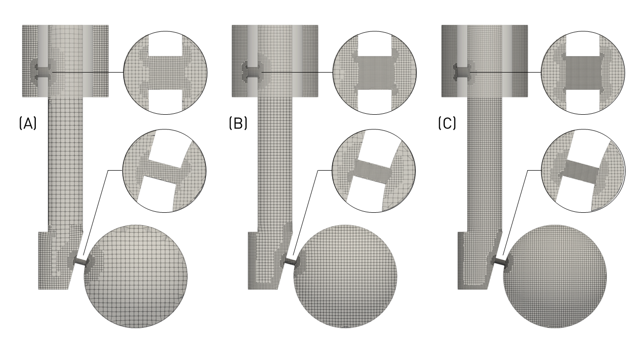
Figure 3: Computational grids employed in the calculations: (a) coarse grid resolution, (b) medium grid resolution, (c) fine grid resolution. A close-up view of the grid resolution in the valve orifice and in the nozzle orifice is shown in the circles.

also included in the model to allow for the mixture flow to exit the de- vice freely. Hexahedral-dominant grids built with the OpenFOAM® util- ity snappyHexMesh are employed for the discretization of the computational domain. In Fig. 3, a cross section of the computational grids with increas- ing resolution employed in the simulations is shown. In the coarse grid of panel 3(a), a minimum and maximum resolution of 250 µm and about 30 µm, respectively, are employed. The grid resolution is increased to a maximum and minimum of 20 µm and 167 µm and to 13 µm and 111 µm in the medium and fine grid, respectively. For the case of turbulent calculation, an addi- tional grid with increased grid resolution at the wall is created, starting from the medium grid resolution. In this grid, three boundary layer cells are added at the wall with increased resolution in the wall-normal direction, ranging from about 20 µm in the stem region to about 5.5 µm in the nozzle orifice region. The total cell count of the computational grids is about 70k, 180k and 580k cells for the coarse, medium and fine grid, respectively.

3.5. Numerical Method

The OpenFOAM® solver compressibleInterFoam for compressible, non- isothermal immiscible fluids, adopting the Volume-Of-Fluid interface captur- ing approach for the representation of the liquid/vapor mixture flow, is employed in the calculations. The model equations (2)-(5) are discretized on the computational grid using second-order accurate schemes in space. For the convective and diffusive transport terms of the momentum equation and energy equations (3) and (4), a linear-upwind and a central-linear scheme are used, respectively. A cell-limited Green-Gauss based reconstruction of cell- centered gradients is used in the linear-upwind scheme to improve numerical stability. For the convective term of the volume fraction equation (5), the scheme of Van Leer is adopted. The numerical integration in time of the model equations is performed using a first-order implicit Euler scheme and an adjustable time-stepping technique, where a variable times-step size ∆t is cal- culated at run-time based on a maximum Courant number Co = U∆t/∆x of 4 inside the liquid and vapor regions and of 2 at the interface between phases, where U and ∆x are local mixture velocity and grid resolution, respectively.

The average time-step size during a metered discharge calculation is about 1.5×10−4 ms, thus an accurate integration in time of the flow governing equa- tions is expected despite the first-order scheme employed in the simulations.

The computational effort for the simulation of a single metered discharge of 350 ms ranges from 5 hours for the coarse grid to 27 hours for the fine grid in parallel execution of the code on 192 and 384 cores, respectively.

4. Results And Discussion

The results of the present work are presented starting from a qualitative analysis of the simulated metered discharge, followed by an assessment of results sensitivity to the main modeling parameters, such as the flash-boiling model coefficients, the grid resolution, temperature dependent properties of the mixture and turbulence modeling. The measurements of mixture density and liquid/vapor flow rates at the nozzle orifice reported by Mason et al.

for the same device geometry and operating conditions are mainly adopted to validate the numerical solution. Other experimental studies for devices with similar geometrical parameters and/or conditions of the metered discharge are employed to evaluate more general behavior of the present numerical model.

14

All the calculations are started from the same initial state, where the propellant is virtually stored in the metering chamber volume by setting the local liquid volume fraction to αl = 1. The initial propellant pressure and temperature in the metering chamber are set to 5.9 bar and 20 ◦C. In the remaining of the computational domain, i.e. the valve orifice, expansion chamber, nozzle orifice and outlet plenum, pressure and temperature are initialized to 1 bar and 20 ◦C and the liquid volume fraction to αl = 0, corresponding to pure vapor. Such condition does not represent the initial state of the actual device, which is initially filled with air. Nonetheless, the displacement of air by the incoming mixture flow is very rapid and usually neglected in system models as well . The modeling of the device actuation, where the metering chamber moves initially with respect to the valve stem until the valve orifice is in full contact with the propellant, is also neglected in the present study, where no partialization of the valve orifice is considered.

The profiles of monitored variables during the simulated metered dis- charge are obtained by averaging the numerical solution in the volume of the device components with a sampling rate of 1 × 10−2 ms. In the case of the nozzle orifice, where high-scattering is observed due to the local high-speed flow, a moving average is applied to extracted profiles using a window of 103 samples.

4.1. Qualitative analysis of simulated metered discharge and comparison with

Experimental Visualizations

In this section, a qualitative analysis of the simulated metered discharge is carried out via the contour maps of liquid volume fraction. The fine grid resolution is employed in the calculation and the coefficients of the flash- boiling model (Cv = 0.0375 and Cc = 240) set from the calibration study against measured data presented in Section 4.2. Constant mixture properties, including the saturation pressure, are adopted in the calculation and the effect of latent heat on the energy equation neglected at this stage. As it will be shown later in the paper, the qualitative results presented here are not altered significantly by the main modeling parameters. Therefore, the analysis can be assumed of general validity in the context of the present model.

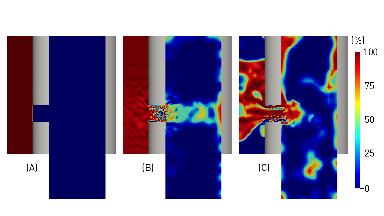
In Fig. 4, the evolution of the liquid fraction field in the valve orifice region is shown at the early stage of the metered discharge. The contour map at t = 0 ms in panel (a) shows the initial condition of the calculation,

15

where the propellant is stored inside the metered chamber above the satura- tion pressure and exposed instantaneously to the valve orifice volume, set to atmospheric pressure. After few instants (t = 0.3 ms), the abrupt formation of vapor can be observed in the orifice volume in panel (b) due to the onset of the flash-boiling, generating a two-phase jet flow from the valve orifice towards the expansion chamber. The impingement of the jet flow on the op- posite side of the valve stem can be also noticed, with partial condensation of the mixture at the stagnation point and the subsequent formation of a liquid film at the wall due to the effect of surface tension. The same panel also shows the perturbations associated with flash-boiling in the valve orifice traveling upstream into the metering chamber volume, triggering the local phase-change process and the initial reduction of the liquid volume fraction.

At t = 30 ms from the start of the metered discharge, the intensity of the jet flow is greatly reduced, as shown in Fig. 4(c), and large scale structures of liquid and vapor are formed and released inside the expansion chamber.

Because of the jet impingement at the wall, some structures travel directly down the valve stem towards the sump region whereas some others moves initially upstream, causing some liquid accumulation in the upper region of the stem. Large voids occupied by the vapor phase are found at this stage inside the metering chamber volume.

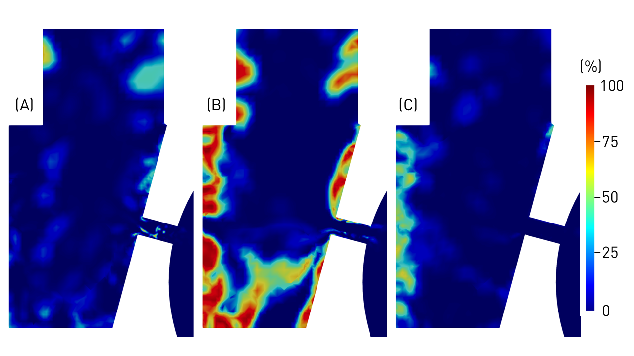
The evolution of the liquid fraction in the sump region from the initial to the final stage of the metered discharge is presented in Fig. 5. In the startup phase (t = 1.5 ms), shown in panel (a), high vapor-quality structures can be seen entering and filling up the sump volume, as well as structures with high liquid volume fraction already entering the nozzle orifice. At t = 30 ms, liquid accumulation in the sump volume due to flow recirculation is observed in Fig. 5(b), along with a thick liquid film forming around the inlet section of the nozzle orifice. In the decay phase of the metered discharge (t = 150 ms), shown in Fig. 5(c), a region of stagnant liquid in the back wall of the sump is found. At this stage, only high vapor quality structures can be seen entering the nozzle orifice.

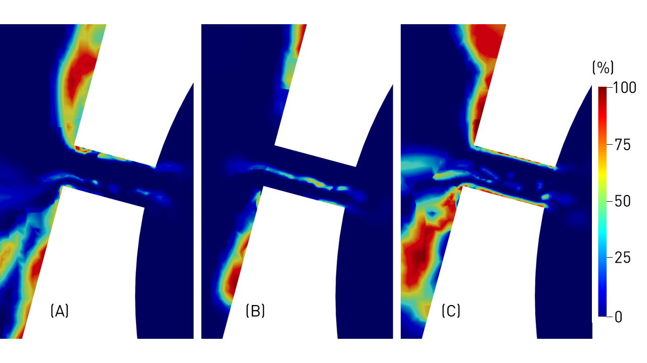
A close-up view of the mixture flow in the nozzle orifice is presented in Fig. 6. In this region, the liquid and vapor structures experience a strong acceleration by moving from the low-speed, recirculating flow in the sump volume to the high-speed flow inside the nozzle. Here, the liquid structures also experience significant stretching, as shown by the elongated shape ap- pearing at t = 60 ms in Fig. 6(b). Fig. 6(a) and Fig. 6(c) also show the formation of a liquid film on the wall surface of the nozzle orifice due to the

16

Figure 4: Temporal evolution of the liquid fraction in the valve orifice region during the startup phase of the metered discharge: (a) t=0 ms, (b) t=0.3 ms, (c) t=30 ms. Figure 5: Temporal evolution of the liquid fraction in the sump region from the startup to the decay phase of the metered discharge: (a) t=1.5 ms, (b) t=30 ms, (c) t=150 ms.

17

Figure 6: Temporal evolution of the liquid fraction in the nozzle orifice region in the intermediate phase of the metered discharge: (a) t=30 ms, (b) t=60 ms, (c) t=90 ms. ingestion of the liquid film formed on the front wall of the sump, co-existing with the liquid and vapor structures traveling into the core region of the orifice.

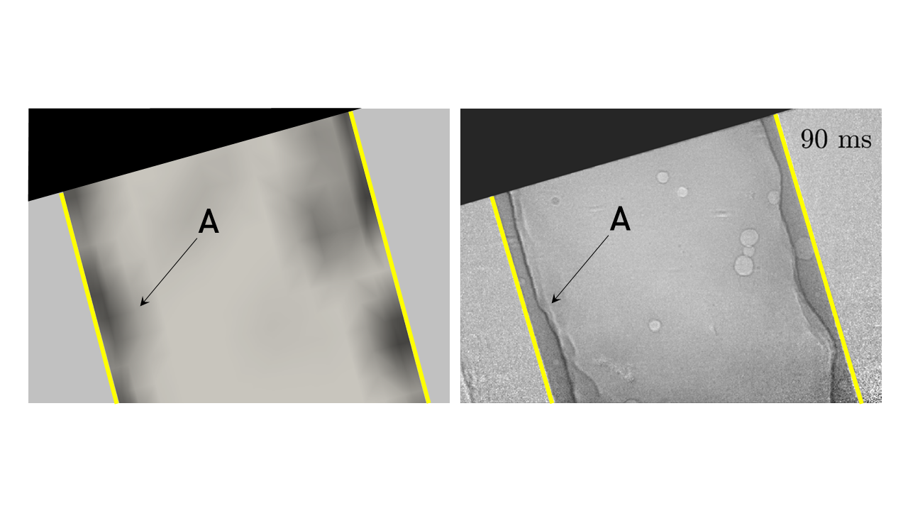
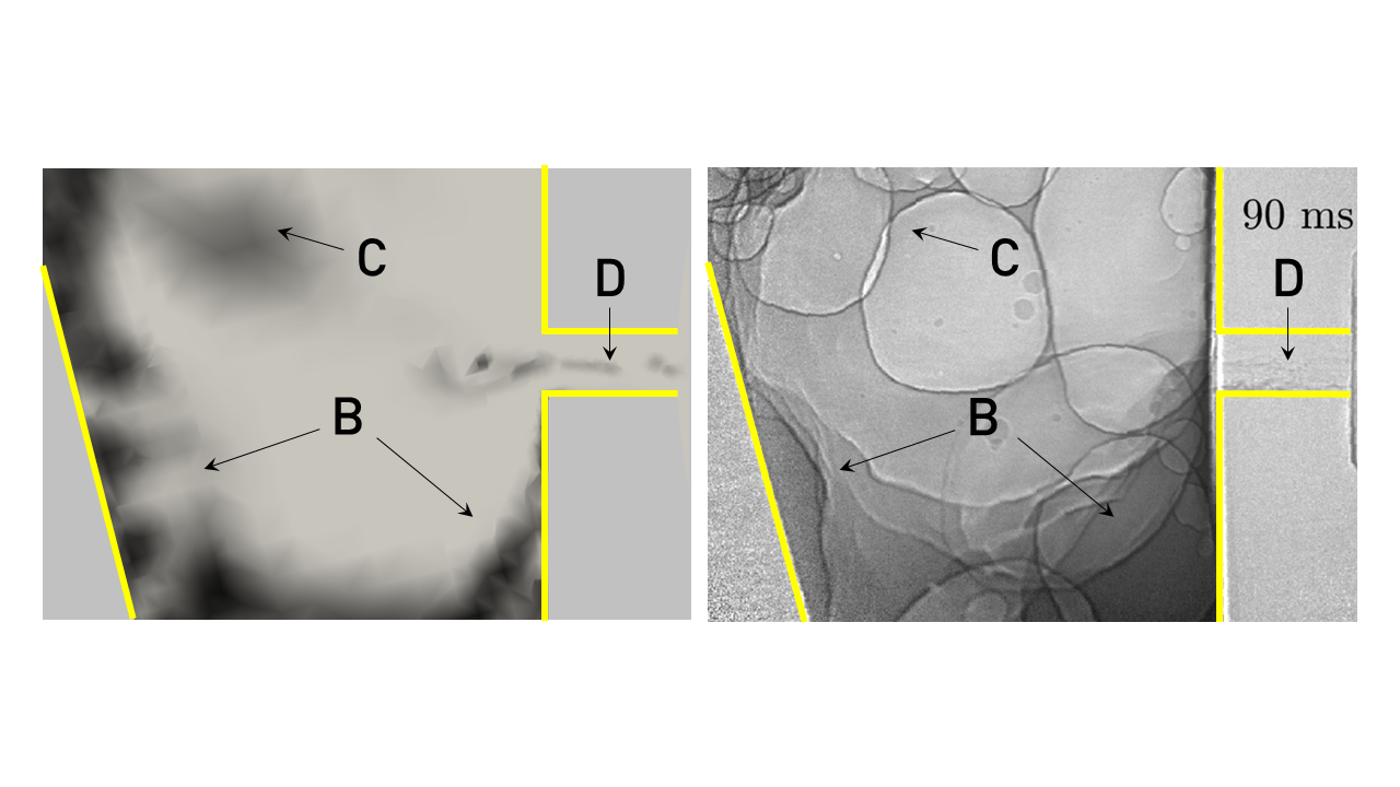
In Fig. 7, a qualitative comparison of the present numerical solution with the experimental X-Ray visualizations of Mason-Smith et al. is presented to assess the capability of the CFD model to provide a realistic representation of the metered discharge. In the picture, the liquid volume fraction is shown in grayscale for the sake of comparison with the X-Ray images. Although the grid resolution is not sufficient to capture its actual thickness, the wall liquid-film predicted by the CFD model on the valve stem surface (detail A in the figure) is also present in the experimental visualizations. On the other hand, the similarity of the numerical solution with the X-Ray visualization in the sump region is quite remarkable.

The Liquid Accumulation In The

bottom part of the sump shown by the CFD model (detail B in the figure), particularly in the lower-right corner, can be clearly seen in the experiment. Moreover, even though the VOF model and the grid resolution employed in the computation are unable to properly resolve the vapor-liquid interface, the presence of large-scale vapor structures is also seen in the X-Ray image (detail C in the figure). The liquid ligaments formed in the nozzle (detail D

18

Figure 7: Comparison of computed liquid volume fraction field (left) with X-ray visu- alizations (right) in the valve stem (top) and sump (bottom) regions (X-ray images are extracted from the original movie courtesy of Mason-Smith et al. ): (A) wall-film for- mation in the stem, (B) formation of large vapor structures in the core of the sump, (C) liquid recirculation and accumulation in the bottom part of the sump, (D) liquid ligaments undergoing acceleration and stretching in the nozzle orifice.

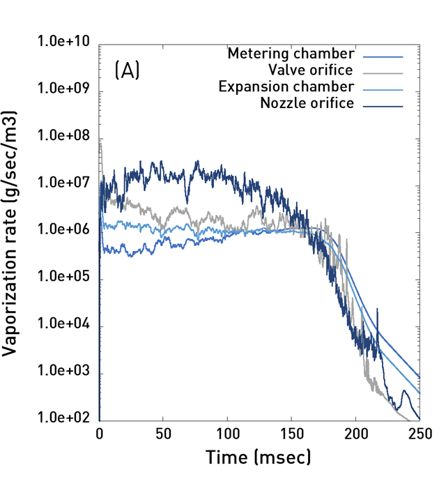
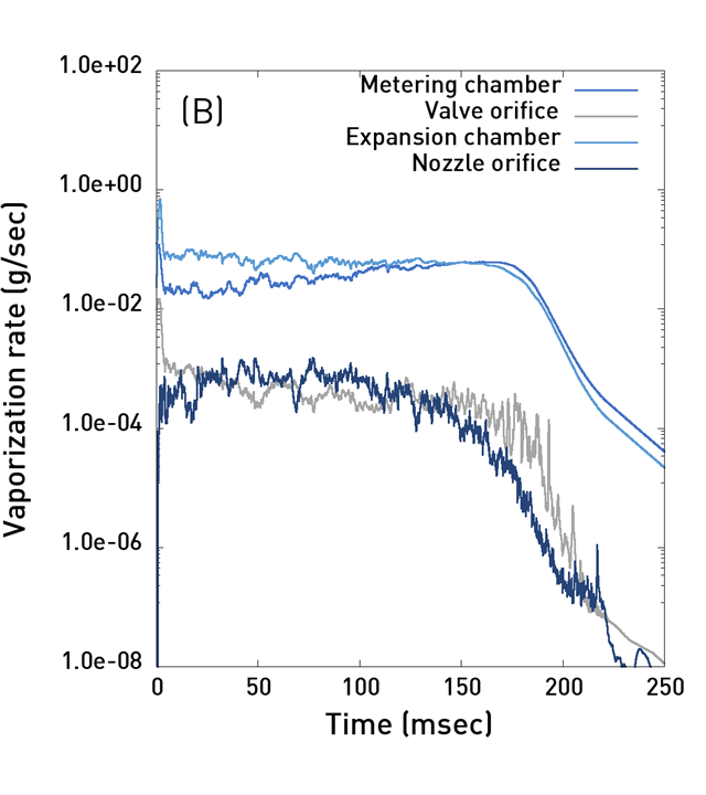
in the figure) are also highlighted clearly by the X-Ray visualizations. The intensity of the flash-boiling and vapor production associated with device components is analyzed in Fig. 8 by plotting the volume-averaged and volume-integrated source term of the liquid volume fraction equation (5) dur- ing the metered discharge. The volume-averaged vaporization rate, presented in panel (a), shows that in the very early stage of device operation (t < 3 ms), the maximum intensity of flash-boiling takes place in the valve-orifice.

However, as the mixture reaches the nozzle orifice, the intensity of the local flash-boiling is found an order of magnitude higher compared to the other device components due to the significant pressure reduction associated with the high-speed flow through the nozzle. On the other hand, the intensity

19

Figure 8: Vaporization rate associated with the main device components: (a) volume- averaged vaporization rate, (b) volume-integrated vaporization rate. of the flash-boiling in the valve orifice rapidly decreases reaching the same order of magnitude as in the expansion and metering chambers at t ≈50 ms. However, the volume integral of the vaporization rate in panel (b) shows that the amount of vapor produced by the two chambers is significantly larger compared to the two orifices.

4.2. Calibration Of The Flash-Boiling Model

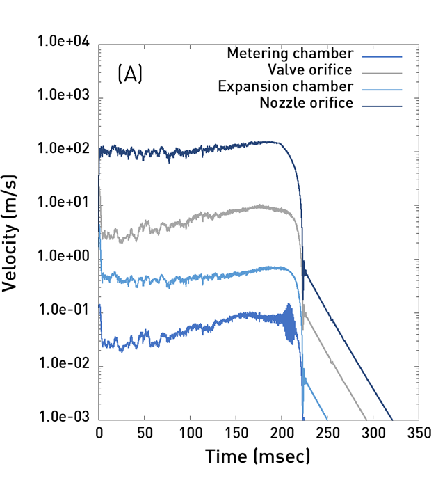
The Kunz model adopted in the present work to account for the flash- boiling phenomenon belongs to a class of phase-change models mainly devel- oped for the simulation of external cavitating flows. In this type of flows, the characteristic velocity and temporal scales U∞and t∞in the model equa- tions (12) and (13) can be clearly associated with the main flow and thus easily identified. In the case of a two-orifice system as the pMDI, even if neg- ligible mean flow speed is observed in the metering and expansion chamber (see Fig. 9(a)), the characteristic flow scales can be either associated with the valve or the nozzle orifice. Despite the higher intensity of the flash-boiling taking place in the nozzle-orifice highlighted by Fig. 8(a), the valve-orifice flow has been selected to compute the characteristic scales, the focus of this

20

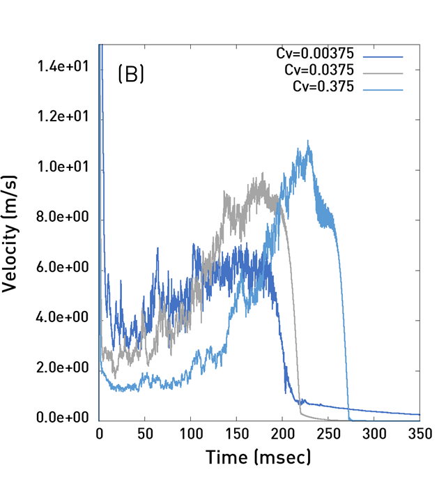
Figure 9: Mixture flow velocity profiles during metered discharge: (a) comparison among the main device components with Cv = 0.0375, (b) effect of evaporation coefficient on velocity profiles in the valve orifice volume.

work being directed towards the flow inside the pMDI and not on the gener- ation of the spray and aerosol downstream of the nozzle orifice. The main calibration of the flash-boiling model coefficients presented here has been conducted using the coarse grid resolution and constant mixture properties. Further evaluations and adjustments have been performed during the sensitivity analysis to the main model parameters starting from the values identified at this stage of the model development, particularly for the case of variable saturation pressure (see Section 4.4). From a preliminary assessment of the mixture velocity in the valve orifice volume, the characteristic velocity and temporal scales have been set to U∞= 2.5 m/s and t∞= 10−1 ms with t∞= Lvo/U∞, where Lvo is the length of the valve orifice. Subsequently, the model coefficients have been varied starting from the standard values of Cv = 100 and Cc = 100 suggested in the work of Kunz , and the numerical solution evaluated by comparing the computed mixture density and liquid and vapor flow rates in the nozzle orifice with the measurements of Mason-Smith et al. . From preliminary calibration tests, it was found that the condensation coefficient has minimal effect on the numerical solution due to negligible condensation rate during the metered discharge where, in

21

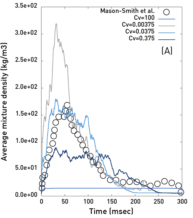
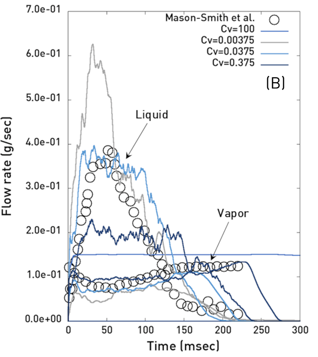
Figure 10: Comparison of computed mixture discharge profiles at the nozzle orifice with the measurements of Mason-Smith et al. : (a) mixture density, (b) liquid and vapor flow rates.

contrast to cavitating flows, no significant pressure recovery takes place. For this reason, once an optimal value was found for Cc only the evaporation coefficient was further evaluated.

Fig. 10 shows the effect of varying the evaporation coefficient on the pre- dicted mixture flow in the nozzle orifice. Using the standard coefficients, the flash-boiling is so intense to make the liquid evaporating entirely across the valve orifice, leading to a single-phase vapor flow in the expansion cham- ber and through the nozzle orifice. A very different value of Cv = 0.0375, along with Cc = 240, gives a good prediction of measured peak values of mixture density and liquid flow rate, whereas the experimental profiles are found overpredicted to some extent in the start-up and decay phases of the metered discharge. On the other hand, the profile of vapor flow rate is found mostly underestimated during the shot. Nonetheless, the overall agreement with the experimental profiles is remarkable given the level of complexity associated with the flash-boiling flow inside the pMDI.

By increasing/decreasing the evaporation coefficient by an order of mag- nitude, the peak values of mixture density decrease/increase by -50%/+100% and those of liquid flow rate by -50%/+50%, respectively, whereas the max-

22

imum relative change in vapor flow rate is +36%/-36%. From the mixture density and liquid flow rate profiles, a more defined peak in the shot is ob- served with decreasing values of the evaporation coefficient, also leading to a better agreement with measurements in the decay phase of the metered discharge, while a non-monotonic behavior is found in the start-up phase.

A significant effect on the duration of the shot, of about 50 ms, is also seen from the vapor flow rates profiles when moving from the optimal coefficient of Cv = 0.0375 to Cv = 0.375. It is also interesting to note that the pre- dicted time of the peak in the shot is fairly insensitive to the calibration of the flash-boiling model and is in good agreement with the experiments. The a-posteriori evaluation of mixture velocity in the valve orifice volume, shown in Fig. 9(b), reveals similar values up to the decay phase of the shot in the range Cv = 0.00375 −0.0375, whereas a more significant velocity variation is found for Cv = 0.375. The use of a constant set of characteristic scales for the flash-boiling model thus seems a reasonable assumption.

4.3. Grid Sensitivity Analysis

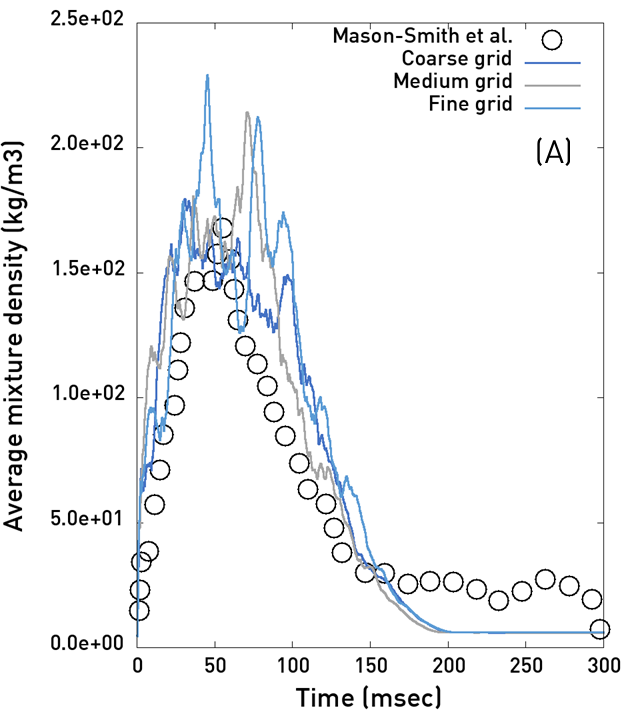
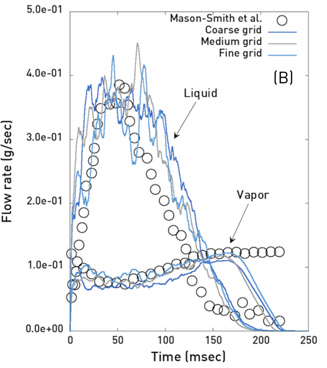
The effect of grid resolution on the computed metered discharge has been evaluated for the case of constant mixture properties and using the flash- boiling model coefficients identified in Section 4.2, giving the best agreement with experimental data (Cv = 0.0375, Cc = 240). In Fig. 11, the computed profiles of mixture density and liquid and vapor flow rates at the nozzle orifice using the coarse, medium and fine grid are compared to the experimental profiles of Mason-Smith et al. . A marginal effect is observed on mixture density, where slightly higher fluctuations are found in peak values moving from the coarse to the medium and fine grid resolutions, without a significant change in the predicted profile. The grid resolution seems to have no effect on predicting the plateau of the mixture density observed in the experiments between 150 and 300 ms, followed by a sudden drop to the vapor density value. However, a notable improvement can be seen in the predicted profiles of liquid and vapor flow rates along the entire metered discharge when moving to the fine grid resolution, with a significant reduction of the overestimated liquid flow rate and, conversely, of the underpredicted vapor flow rate.

The increased accuracy in the predicted flow rates at the nozzle orifice with increasing grid resolution is quantified and shown in Fig. 12, where the computed mass of liquid and vapor ejected during the metered discharge, given by the integral of the flow rate profiles, is compared to values measured in the experiments of Mason-Smith et al. . A systematic improvement is

23

Figure 11: Impact of grid resolution on the computed mixture discharge profiles at the nozzle orifice: (a) mixture density, (b) liquid and vapor flow rates. observed when moving from the coarse to the fine grid resolution, with the error in the computed ejected mass dropping from +32% to +20% for the liquid phase and from -26% to -12% for the vapor phase, respectively. The results also show the finest grid resolution employed in this study does not allow to reach a fully-converged prediction of the ejected mass, for which a variation of -5% and +14% is still observed between the medium and fine grids. Nonetheless, since the scope of the present work is the development of a numerical model for industrial applications, where the computational cost of the simulations must be limited, and no significant changes and shifts in the overall shape of the predicted profiles in Fig. 11 can be noticed, we deem the analysis presented in this section sufficient to assess the robustness of the numerical model.

The effect of grid resolution on the simulated metered discharge is further investigated in Fig. 13 by the analysis of the global vaporization rate inside the pMDI and of the mixture velocity in the nozzle orifice. The increased mixture velocity with increasing grid resolution in Fig. 13(b) supports the improvement in the predicted vapor flow rate, but appears in contrast with the predicted liquid flow rate, which is found decreasing with increasing grid resolution. However, the profiles of global vaporization in Fig. 13(a) shows

Related Journal Articles & DOI Links

Selected peer-reviewed publications relevant to 12 Lead ECG Acquisition. Click the DOI to access the full paper (may require institutional access).

Why Choose Us?

Bangalore guidance for robotics, Spectre and autonomous systems projects.