Raspberry Pi Medical Imaging

Automatic Landmarks Correspondence Detection in Medical Images with an Application to Deformable Image Registration Monika Grewala,*, Jan Wiersmab, Henrike Westerveldb, Peter A. N. Bosmana,c, Tanja

Alderliestend

aEvolutionary Intelligence Research Group, Centrum Wiskunde & Informatica, 1098 XG, Amsterdam, The

Delft, The Netherlands

Abstract. Purpose: Deformable Image Registration (DIR) can benefit from additional guidance using corresponding landmarks in the images. However, the benefits thereof are largely understudied, especially due to the lack of automatic landmark detection methods for three-dimensional (3D) medical images.

Approach: We present a Deep Convolutional Neural Network (DCNN), called DCNN-Match, that learns to predict landmark correspondences in 3D images in a self-supervised manner. We trained DCNN-Match on pairs of Computed Tomography (CT) scans containing simulated deformations. We explored five variants of DCNN-Match that use different loss functions and assessed their effect on the spatial density of predicted landmarks and the associated matching errors. We also tested DCNN-Match variants in combination with the open-source registration software Elastix to assess the impact of predicted landmarks in providing additional guidance to DIR.

Results: We tested our approach on lower-abdominal CT scans from cervical cancer patients: 121 pairs containing simulated deformations and 11 pairs demonstrating clinical deformations. The results showed significant improvement in DIR performance when landmark correspondences predicted by DCNN-Match were used in the case of simulated (p = 0e0) as well as clinical deformations (p = 0.030). We also observed that the spatial density of the automatic landmarks with respect to the underlying deformation affect the extent of improvement in DIR. Finally, DCNN-Match was found to generalize to Magnetic Resonance Imaging (MRI) scans without requiring retraining, indicating easy applicability to other datasets.

Conclusions: DCNN-Match learns to predict landmark correspondences in 3D medical images in a self-supervised manner, which can improve DIR performance. Keywords: Deformable Image Registration, Computed Tomography, landmarks detection, Deep Learning.

1 Introduction

Deformable Image Registration (DIR) is a task of aligning a source (or moving) image to a target (or fixed) image by optimizing a Displacement Vector Field (DVF). The aligned source image can then be computed by resampling the source image at the spatial locations specified by the map- ping. DIR has tremendous application possibilities in the radiation treatment workflow required

Arxiv:2109.02722V2 [Cs.Cv] 21 Feb 2023

for cancer treatment e.g., automatic contour propagation,1,2 dose accumulation.3–5 However, DIR in regions such as the pelvis is challenging due to large local deformations and appearance dif- ferences caused by physical processes such as bladder filling, and the presence of gas pockets and contrast agents.2 In such DIR scenarios, the existing non-linear intensity-based registration approaches6–8 often get stuck in a local minimum.4 Many previous studies9–14 have shown that landmark correspondences between the images to be registered can provide additional guidance to the intensity-based DIR methods and help overcome local minima. However, to the best of our knowledge, such an approach has not been tested on pelvic scans.

Manual annotation of landmarks for DIR in the clinic is not practically tractable due to two main reasons. First, a high number of landmarks is desired, and it is difficult to unambiguously define such a high number of landmarks manually. Second, manual annotations require lots of time from clinicians, which is hardly available. Therefore, an automatic method for finding landmark correspondences is required. Although many endeavours have been made in the direction of auto- matic landmarks correspondence detection in medical images,14–16 there remain significant gaps to fill. The existing methods usually employ large pipelines consisting of multiple components, each component using multiple hyperparameters derived from image features specific to the underlying dataset. Consequently, the entire pipeline is sensitive to small variations in local image intensi- ties and choices of hyperparameters, making application to a new dataset difficult. Moreover, in datasets such as pelvic scans with ill-defined boundaries between soft tissues, intensity gradient based landmark detection may not work at all.

Convolutional Neural Networks (CNNs) are known to learn deep features from images, which are robust to small variations in local image intensities. In recent years, deep CNNs have not only shown remarkable performance in difficult computer vision tasks in medical imaging,17,18 but also

2

good generalization to unseen data. Moreover, with the advances in the available computational resources, CNN-based solutions turn out to be faster than their traditional counterparts. There- fore, there is a strong motivation to replace the entire pipeline for automatically finding landmark correspondences by a deep CNN. Recently some deep CNN methods have been developed for au- tomatic landmark detection in medical images,19–21 but these are limited to either 2D datasets or supervised learning of a few manually annotated landmarks. Other relevant works include methods for landmark propagation from a template image by learning pixel-wise anatomical embeddings22 or through deformable image registration.23 While such methods allow for single shot landmark detection in a new image, the requirement of manual annotation of landmarks on the template im- age still exists. Another study uses unsupervised image registration as a proxy task to discover landmarks shape descriptors,24 but this method is limited to discovering a small number of land- marks (∼100 landmarks per image pair).

In this study, we present a deep CNN (referred to as “DCNN-Match”) for automatic landmarks correspondence detection (i.e., simultaneous landmark detection as well as matching) in 3D im- ages. The presented method is an extension of our method for 2D images.21 Briefly, the neural network is trained on pairs of 3D lower abdominal Computed Tomography (CT) scans such that the network learns to predict landmarks at salient locations in both the images along with the cor- respondence score of each landmark pair. One key feature of the presented method is that unlike supervised methods, the neural network in the presented method is trained in a self-supervised manner without using any manual annotations. This is important because manual annotations on medical images are not always readily available, mainly because it is time-consuming to create them.

It is essential to investigate the added value of automatic landmarks correspondence detection

3

towards the improvement of the DIR solutions to estimate the potential deployability of landmarks- guided DIR approaches in the clinic. Existing studies have investigated the added value of auto- matic landmark correspondences towards DIR independently of the underlying automatic land- mark detection method.10,11,14 Since change in the automatic landmarks correspondence detection method changes the aspects of the automatic landmarks e.g., spatial distribution and matching ac- curacy, the effect of the automatic landmarks on the DIR performance is likely to be affected as well. Therefore, we believe that developing a method for automatic landmarks correspondence detection and at the same time integrating it with a DIR pipeline can provide numerous insights.

To this end, we have integrated our method for automatic landmark detection and matching with an existing DIR software so that the added value of using landmark correspondences in solving DIR problems can be assessed. Further, we investigate five different variants of the developed method by use of different loss functions during training that each predict landmark correspondences with different spatial distributions and matching errors, to assess the effect of different types of au- tomatic landmark correspondences towards the improvement of DIR. The present work has the

Following Contributions:

• We extended our previously published end-to-end self-supervised deep learning method for automatically finding landmark correspondences in medical images from 2D to 3D. The key

Highlights Of The Method Are:

– the method does not set any prior on the definition of landmarks – the method does not require manual annotations for training • We integrated our automatic landmark correspondence detection method in 3D (DCNN- Match) with an open-source registration software Elastix6,25 to develop a DIR pipeline that

4

utilizes additional guidance information from automatic landmark correspondences. We used this DIR pipeline to investigate the added value of automatic landmark correspondences in providing additional guidance to the DIR method and finding better DIR solutions.

• We varied the landmarks correspondence detection method and investigated how it affected the added value to the DIR method. We explored five different variants of the proposed automatic landmarks correspondence method.

• We experimentally investigated the generalization capability of our proposed automatic land- marks correspondence detection method to a Magnetic Resonance Imaging (MRI) dataset.

2 Materials And Methods

In the following sections, we describe DCNN-Match (section 2.1), and the DIR pipeline which uses the information from automatic landmark correspondences predicted by DCNN-Match to guide the registration (section 2.2). Sections 2.3 and 2.4 provide details of implementation and hy- perparameters for reproducibility. Sections 2.5, 2.6, 2.7, and 2.8 describe the datasets, experiments, evaluation metrics, and statistical testing used in the experiments, respectively.

2.1 Dcnn-Match

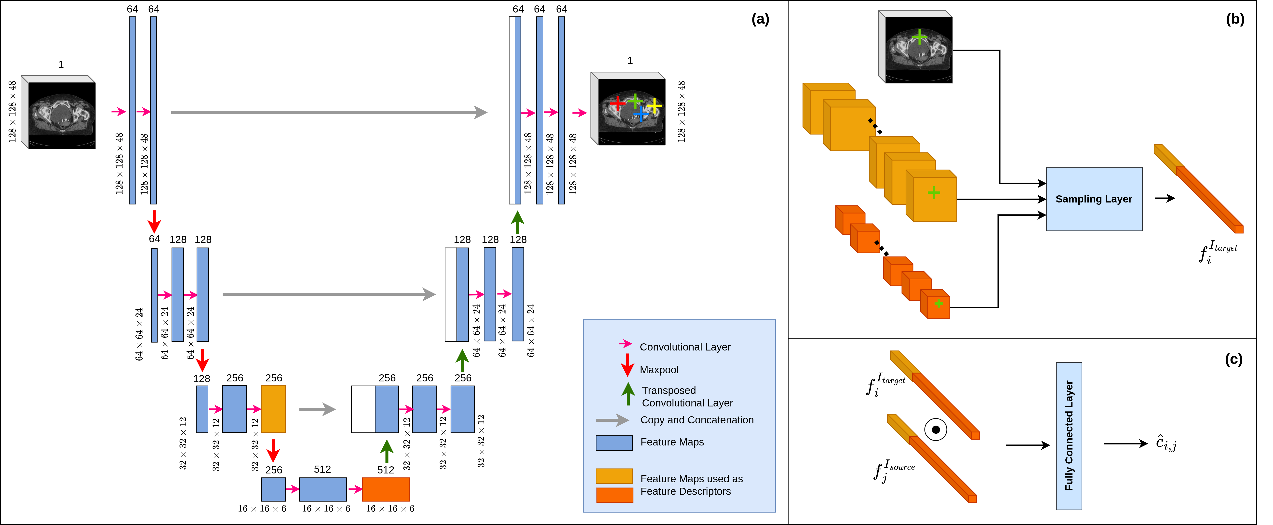
We extended our approach21 for finding landmark correspondences in 2D CT scan slices to work on 3D CT scans. The different components of the 3D approach are illustrated in Figure 1. Briefly, the approach proposed in21 consists of a Siamese network with three modules: a) two CNN branches with shared weights, b) a sampling layer, c) a descriptor matching module. The CNN branches comprise an image-to-image translation network that maps an input image to a feature map. The

5

architecture of the network is derived from the famous UNet architecture26 proposed for image seg- mentation. For a given pair of target image (Itarget) and source image (Isource), the CNN branches predict a landmark probability map describing the probability ˆpIx

I (X ∈{Target, Source}) Of Each

spatial location i being a landmark. The sampling layer is a parameter-free module that samples K (hyperparameter) landmark locations with top landmark probabilities during training. During inference, the sampling layer samples all landmark locations with landmark probabilities above a

Threshold. We Used The Value 0.5, Same As In.21

Additionally, the sampling layer samples a feature vector from the feature maps of the last two downsampling levels in the CNN branch at the coordinates of each ith landmark location

I

by concatenating the sampled feature vectors.

This

allows for efficient use of the network weights by simultaneous learning the landmark detec- tion as well as feature description of each landmark without unnecessarily increasing the net- work size. Moreover, the concatenation of features from different downsampling levels emulates the behavior of multi-scale feature description, which otherwise, is achieved by calculating fea- tures from a Gaussian pyramid representation of the image. Following the calculation of fea- ture descriptors for each landmark location, the sampling layer creates feature descriptor pairs

J

) ∀i = 1, 2, ..., K in Itarget and ∀j = 1, 2, ..., K in Isource to feed to the descriptor matching module. The descriptor matching module predicts the landmark matching probabilities corresponding to each feature descriptor pair.

2.1.1 Self-Supervised Training

The network is trained in a self-supervised manner on pairs of target (Itarget) and source (Isource) lower abdominal CT scans containing simulated deformations. The details on the generation of

6

target and source image pairs are provided in section 2.3. Following the sampling of landmark locations i = 1, 2, ..., K in Itarget and j = 1, 2, ..., K in Isource along with their corresponding feature descriptors f Itarget

J

) are constructed in the sampling layer. The feature descriptor pairs are con- sidered corresponding to all i and j, allowing for feature descriptor matching between far-away locations in the images without requiring encoding of the underlying deformation field explicitly.

Since the simulated deformations used to create source and target image pairs during training can not represent the complex large deformations in a clinical setup exactly, learning the feature de- scriptor matching not explicitly dependent on the underlying deformation field is likely to help the neural network generalize better to clinical scenario.

The ground truth ci,j of the correspondence of each feature descriptor pair is calculated on- the-fly based on the known simulated deformation. Each sampled landmark location in the target image is projected onto the source image based on the known simulated deformation and the near- est predicted landmark (within a distance of 2 voxels = 4 mm) in the source image is considered its match. We used a threshold of 4 mm (instead of image resolution = 2 mm) in order to find a rea- sonable number of landmark matches from random predictions in the beginning of the training to ensure sufficient supervision. the value of ci,j = 1 for matching and ci,j = 0 for non-matching fea- ture descriptor pairs. Subsequently, the ground truth pIx

I For The Landmark Probability Of Landmark

location i in image Ix, x ∈{target, source} is determined as follows:

1

if ∃! j ∈{0, 1, 2, ..., K} in image Iy, y ∈{target, source}, y! = x ∧ci,j = 1

7

The ground truths ci,j are used directly as ground truths for the matching probability of the feature

J

). In other words, the ground truth is generated such that the land- mark probability as well as the descriptor matching probability is high for the matching locations between the two images and low otherwise. The network is trained by minimizing a multi-task

Loss Defined As Follows:

Loss = LandmarkProbabilityLossItarget + LandmarkProbabilityLossIsource

(2)

The LandmarkProbabilityLossIx for the probabilities of landmarks in image Ix, x ∈{target, source}

(3)

where CrossEntropyLoss is the cross entropy loss between predicted landmark probability ˆpIx

And Ground Truth Pix

i of the ith sampled location. K is the total number of sampled landmark loca- tions in image Ix. Further details of the LandmarkProbabilityLoss are omitted for brevity and

Can Be Found In.21

The DescriptorMatchingLoss allows the network to learn feature descriptor matching automat-

Ically And Is Defined As Follows:

DescriptorMatchingLoss = DescriptorHingeLoss + DescriptorCELoss

J

are the feature descriptors corresponding to the ith and jth landmark locations in the input images Itarget and Isource, respectively; ci,j is the ground truth matching probability for the feature descriptor pair (f Itarget

); Mpos And Mneg Are The Margins For The

L2-norm of matching (positive class) and non-matching (negative class) feature descriptor pairs. The Hinge losses corresponding to positive and negative classes are normalized by Kpos (number of positive feature descriptor pairs) and Kneg (number of negative feature descriptor pairs), respec- tively to account for the class imbalance between positive and negative feature descriptor matches.

(6)

where ˆci,j is the predicted matching probability; WeightedCrossEntropy represents the binary cross entropy loss where the loss corresponding to the positive class is weighted by the frequency of negative examples and vice versa.

In the beginning of the training, the predicted landmark probability maps by the CNN branches are random and by chance only a few landmark locations have correct correspondence (i.e., ci,j = 1) between images. The loss defined in (2) encourages high landmark probability at these loca-

9

tions as well as high feature descriptor matching probability for the feature descriptor pairs of these locations and low landmark probability and feature descriptor matching probability other-

Wise. Additionally, The Term (1 −ˆPix

i ) in (3) encourages high landmark probability at all locations i.e., encourages more landmark locations to have correct correspondence in the other image. Con- sequently as the training progresses, the network learns to identify salient locations in the images that have correct correspondence in the other image as well and predicts high landmark probabili- ties at the these locations.

2.1.2 End-To-End

The conventional approach to establish landmark correspondences between an image pair utilizes

The Following Steps:

• Landmark detection, in which landmarks are detected in both the images independently. • Feature description, wherein a vector (often called “descriptor”) is calculated to describe the image properties surrounding the landmark location. An example of a feature descriptor is Scale Invariant Feature Transform (SIFT27), which calculates the histograms of orientations from the image patches of different scales around the landmark.

• Landmark matching, wherein landmark descriptors in both the images are matched using a matching algorithm. A straightforward matching algorithm is brute force matching, which aims at finding the best match among all the landmark locations in the source image for each landmark location in the target image.

Our approach replaces each of the abovementioned components with a neural network module, and connects the neural network modules such that the gradients flow from the end to the inputs.

10

The modules of landmark detection and description are represented by the CNN branches of the Siamese network. The task of landmark matching is performed by the descriptor matching module. It is important to mention that the key feature of DCNN-Match lies in the assembling of different modules to provide a simple end-to-end deep learning solution for simultaneous landmark detec- tion, description, and matching automatically. Therefore, the proposed approach can be easily modified, e.g., it may be improved by the use of a different neural network in any of the modules.

Fig 1: Illustration of the components of DCNN-Match. (a) Illustration of different layers in the shared CNN branch used for landmark detection and feature description. (b) The sampling layer samples the feature maps of the last two downsampling levels in the CNN branch at the locations described by the landmark probability map. (c) The descriptor matching module realized by a fully connected layer predicts the matching probability of a feature descriptor pair.

2.1.3 Extension To 3D Images

We have extended our original approach proposed in21 to work on 3D images by performing three modifications. The first obvious modification was to use 3D convolutional kernels (kernel size = 3 × 3 × 3) instead of 2D convolutional kernels in the CNN branches. The sampling layer and the feature descriptor matching module were also adapted for 5D tensors arising from training on 3D images. The generation of a valid mask during training as described in21 section 2.4 was also

11

adapted for 3D images. The valid mask makes the network learn a content-based prior to predict landmarks only in the regions that include patient anatomy and not in the background or the CT couch.

Second, since we had a considerably large training dataset (details in section 2.5) as opposed to,21 we kept the same number of kernels in each layer as the original UNet architecture.26 Third, we trained the network on 3D patches of the entire CT due to GPU memory constraints. During inference, we evaluated the network on the patches belonging to the same spatial locations in the target and source images. The patches were cut with 50% overlap and the final output combined the predicted landmark pairs in all patches. All the corresponding landmarks predicted in all the overlapping patches were considered landmarks. Using a small patch size restricts the network from learning landmark matches in locations that are far apart in the two images. Therefore, the patch size has to be decided while keeping in mind the spatial extent of deformations we want the network to learn. This is further described in the hyperparameters section 2.4.

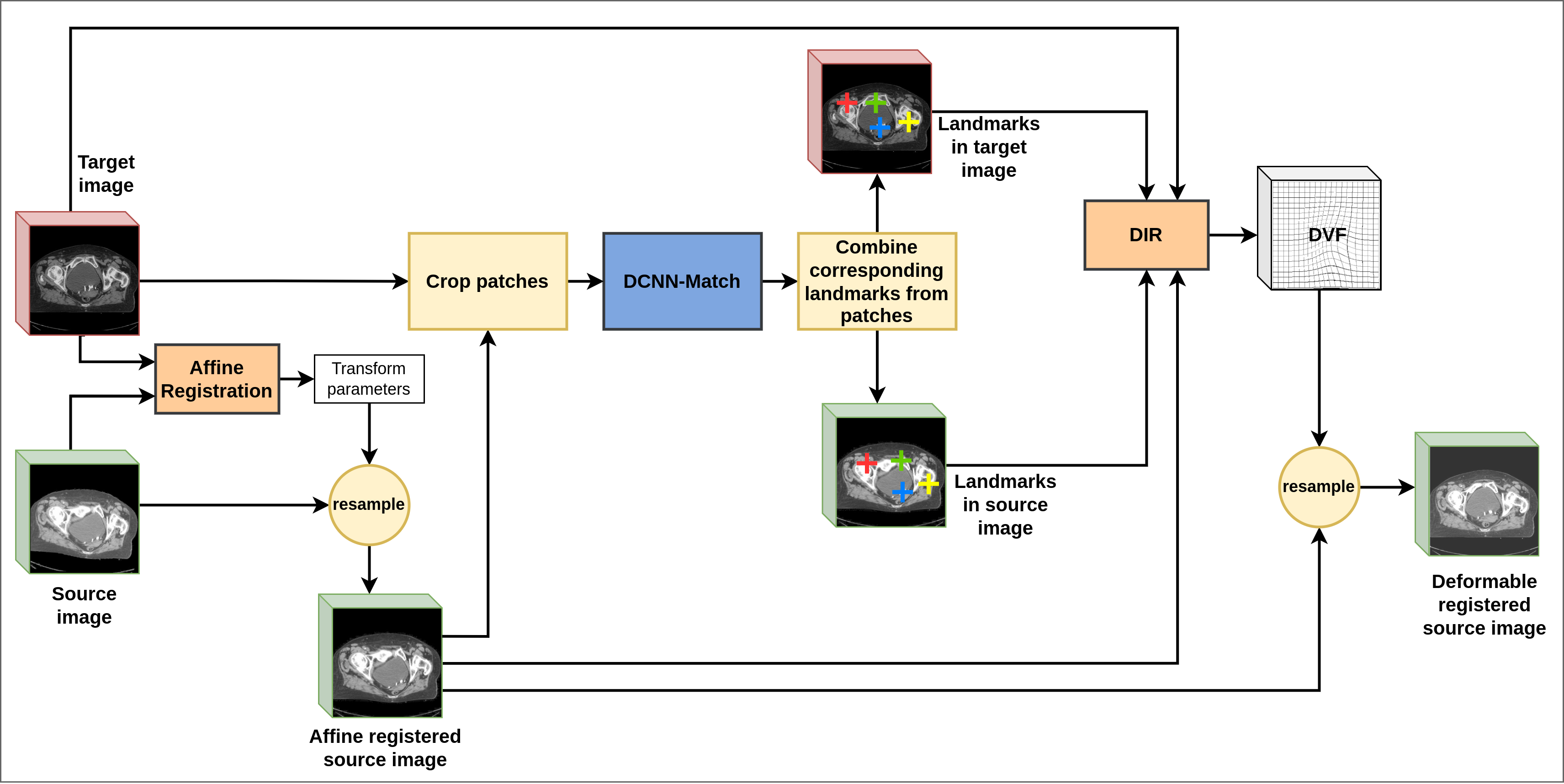
2.2 DIR with Additional Guidance from Automatic Landmark Correspondences We integrated DCNN-Match with the open-source registration software Elastix6,25,28 to create a pipeline for DIR that utilizes the additional guidance information from automatic landmark corre- spondences. A schematic of the DIR pipeline is provided in Figure 2.

DIR requires calculation of a DVF that maps each spatial location in the target image to a spatial location in the source image. In Elastix, the DVF is parameterized by B-splines and the coefficients of B-splines are optimized by non-linear optimization. We align the source CT scans with the target CT scans using affine registration before performing DIR. The parameters of the 3D affine transformation matrix (i.e., translation, rotation, scale, and shear) are optimized by max-

12

Fig 2: DIR pipeline with automatic landmarks correspondence detection using DCNN- Match. The source image is affine registered with the target image followed by automatic land- marks correspondence detection using DCNN-Match. DCNN-Match provides the locations of corresponding landmarks (shown with similar colored cross-hairs) in both the target and affine registered source image. The DIR module finds a DVF by utilizing the additional guidance infor- mation from automatic landmark correspondences. The final transformed (deformable registered) source image is obtained by resampling the affine registered source image according to the ob- tained DVF.

imizing the normalized mutual information between the target and source scans. The target and the affine registered source CT scan are input to the DCNN-Match, which provides the locations of corresponding landmarks in both the scans. The DIR module in Elastix takes the target image, affine registered source image, and the pairs of corresponding landmarks in both the images as input. The DIR is performed by optimizing the following objective function:

13

fGuidance = weight0 AdvancedMattesMutualInformation

+ Weight1 Transformbendingenergypenalty

+ weight2 CorrespondingPointsEuclideanDistanceMetric

(7)

where AdvancedMattesMutualInformation represents the maximization of mutual informa- tion between two scans (for details refer to29), TransformBendingEnergyPenalty is a regular- ization term that penalizes large transformations, and CorrespondingPointsEuclideanDistanceMetric is used for minimizing the Euclidean distance between the landmarks in the target CT and the land- marks in the source CT. weight0, weight1, and weight2 control the relative contribution of each term towards the objective function.

2.3 Implementation

The DIR pipeline was developed in Python. We used the PyTorch framework30 for developing DCNN-Match. The training was done on an RTX 2080 Ti GPU and took approximately 21 hours. The weights of DCNN-Match were initialized using the He norm method.31 The training was done using the Adam optimizer32 with a learning rate of 1e−4. The neural network weights were regularized by using a weight decay of 1e−4.

We randomly cropped 3D patches of dimension 128 × 128 × 48 from the entire CT scan volume and used them as target images. The source images were generated on-the-fly by applying one of the following random transformations on the target images: translation, rotation, scale, or elastic transformations. The magnitudes of the affine transformations along all axes were sampled

14

from the following uniform distributions: U(−12mm, 12mm), U(−20◦, 20◦), and U(0.9, 1.1) for translation, rotation, and scale respectively. The elastic transformations were applied so as to simulate the two types of soft tissue deformations present in the lower abdominal scans: a) large local deformations e.g., bladder filling, b) small tissue deformations everywhere in the image. The large local deformations were simulated by a 3D Gaussian DVF (DV Flarge) of magnitude at center = U(2mm, 24mm) and σ = U(64mm, 128mm) at a random location in the image. The small deformations everywhere in the image were simulated by Gaussian smoothing of a random DVF (DV Fsmall = U(1mm, 12mm)) at each location. DV Flarge and DV Fsmall were additively applied to the target image to generate the source image with elastic transformation.

2.4 Hyperparameters

Apart from the conventional hyperparameters involved in designing and training a DCNN e.g., network depth and width, optimizer, and learning rate, there are two hyperparameters specific to DCNN-Match: patch dimensions and the number of sampling points during training (K). As indicated in the previous section, we used a patch size of 128 × 128 × 48 (256 mm × 256 mm × 96 mm). This way the neural network’s Field-Of-View (FOV) was maximum given the network depth and GPU memory constraints, which ensured that the landmark correspondences could be learned for deformations as large as 128 mm in-plane and 48 mm along the transverse axis. Similar to,21 K = 512 was used based on the visual inspection that the predicted landmarks in the validation set (details in section 2.5.1) covered the image sufficiently.

In Elastix, we used the advanced mattes mutual information as a similarity metric because it has been found successful in earlier studies on DIR.2 For deciding other hyperparameters such as the number of iterations, step size, step decay, weight0, weight1, and weight2, we used the

15

development set (details in section 2.5.1). For this purpose, the pairs of target and source images were generated in a manner similar to the training set. 100 locations were sampled randomly on the target image and their corresponding location in the source image was established by transforming the coordinates with the inverse DVF used for generating the source image. The hyperparameters were tuned based on the following observations on the development set: the transformed source image after registration was not distorted and showed no visible folding, the image alignment at the 100 randomly sampled locations improved after registration. The exact configuration of Elastix used for affine registration and DIR is provided in the Appendix A.

2.5 Data

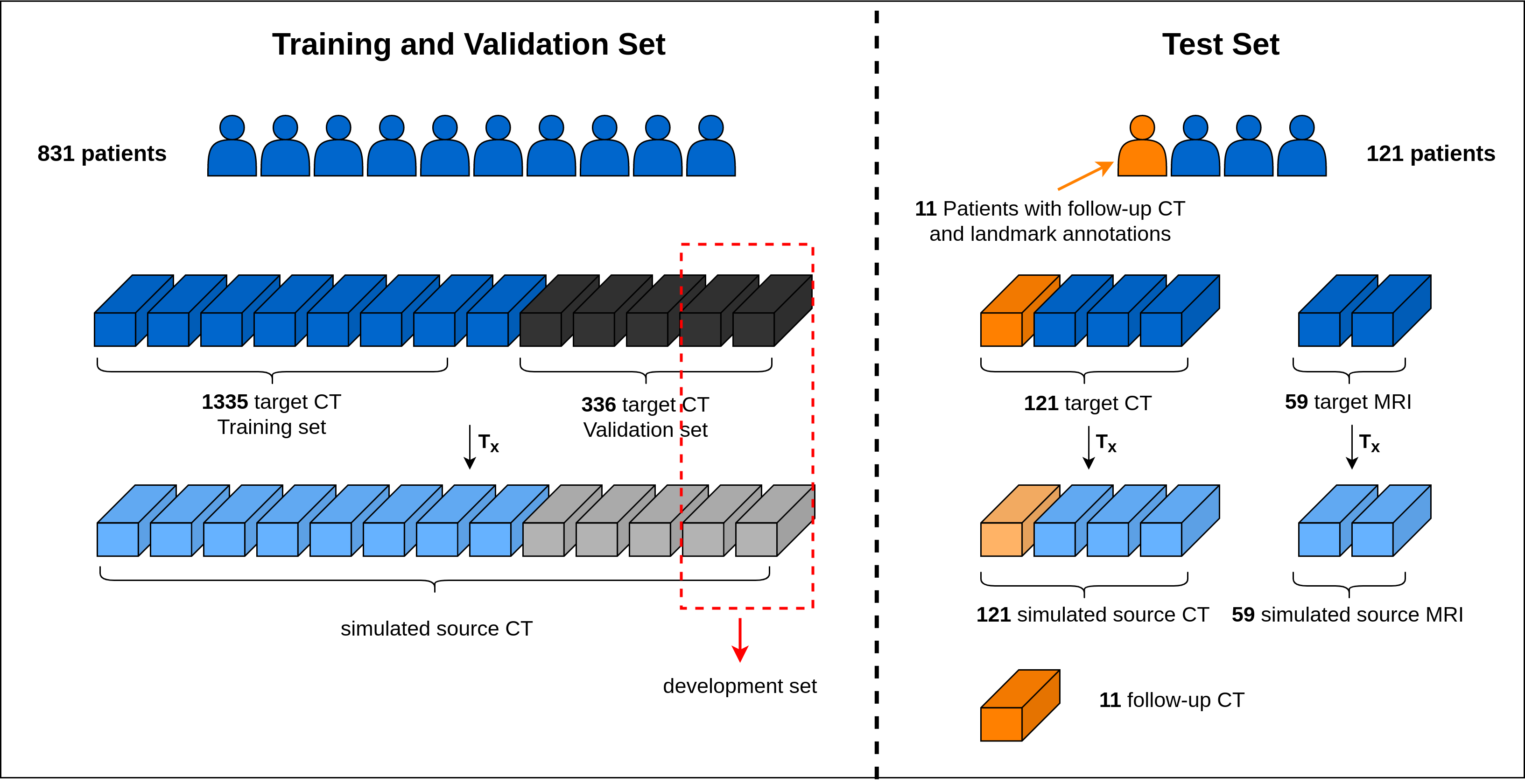
An overview of the data is provided in Figure 3. We retrospectively included the CT and MRI scans from female patients (age range 22 - 95 years), who received radiation treatment in the lower location AMC, the Netherlands. The data was transferred in anonymized form through a data transfer agreement. A subset of these scans was the same as used in a previous study.21

2.5.1 Training And Validation Set

A total of 1671 CT scans of 831 patients were used for developing the approach: 1335 CT scans for training and 336 CT scans for validation. A subset containing 10 CT scans from the validation set (referred to as the development set) was used to tune the hyperparameters of the DIR pipeline.

All the CT scans were resampled to have 2 mm × 2 mm × 2 mm voxel spacing and the image intensities were converted from the Hounsfield units to a range of 0 to 1 after windowing.

16

Fig 3: Data Overview. The vertical dashed gray line depicts the patient-level split between the training and validation set, and test set.

(Left) And Source (Right) Ct

is shown.

Pearance Difference In The

bowel due to contrast.

2.5.2 Simulated Deformations Test Set - Ct

We tested the performance of DCNN-Match and the DIR pipeline on a curated dataset of 121 CT scans belonging to 121 patients, who received radiation treatment for cervical cancer. The

17

mean FOV of acquisition of the CT scans was 546 mm × 546 mm × 368 mm and the scans were resampled to 2 mm × 2 mm × 2 mm voxel spacing. The available CT scans were used as target images and corresponding source images were simulated by applying random elastic transformations to the target CT scans according to the method described in the section 2.3 above.

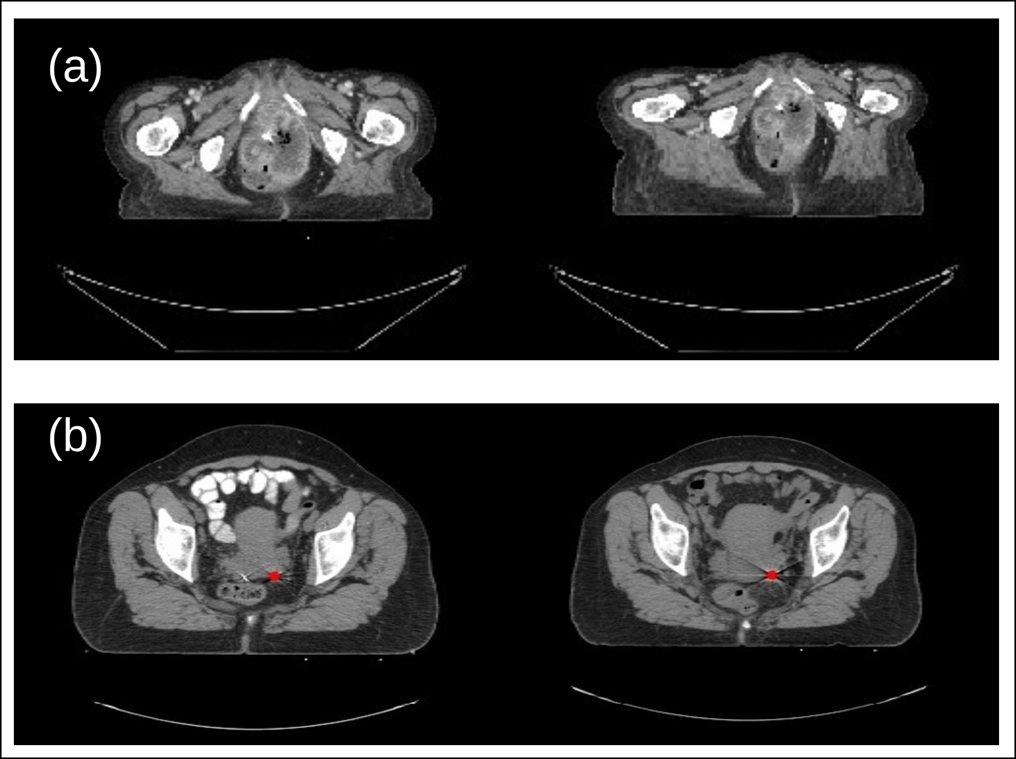
Further, an example of the simulated deformation and the obtained source CT is shown in Figure 4 (a). In each pair of target and source image, 100 corresponding locations were sampled with uni- form random distribution. These sampled locations were used as validation landmarks for assess- ing the performance of DCNN-Match and the DIR pipeline.

2.5.3 Clinical Deformations Test Set - Ct

The CT scans in a clinical setup exhibit complex bio-mechanical deformations including discon- tinuities in the deformation field around sliding tissues and large deformations that may not be Gaussian. The random Gaussian DVF used for deforming the images to obtain a simulated test set is an oversimplification of the underlying situation. Therefore, it is essential to investigate if the observations on the simulated deformations test set hold in the clinical setting as well. To this end, additional CT scans (referred to as follow-up scans) were searched in the clinical database for a subset of patients in the test set (11 patients). The first CT scans from these patients were used as target images and the corresponding follow-up CT scans were used as source images.

Corresponding landmarks at 29 locations were manually identified in each target and source CT scan by a clinical expert. These landmarks included six fiducial markers in the vaginal wall, and anatomical landmarks e.g., aortic bifurcation, cervical os, and os coccygis. Since clinically available scans were used, the number of fiducial markers were different in each patient in ac-

18

cordance with the treatments given to the patients. The majority of the patients’ scans had three fiducial markers, while some had less or more. If a patient’s scan had less than three fiducial mark- ers, calcification (if present) in corresponding anatomical locations were used as landmarks. If a patient’s scan had more than three fiducial markers, only three of them were used. An example landmark location is shown in Figure 4 (b) and the complete list of landmark locations is provided in Appendix B.

2.5.4 Simulated Deformations Test Set - Mri

MRI scans of 59 cervical cancer patients (subset of the 121 cervical cancer patients mentioned in section 2.5.2, who received brachytherapy treatment) acquired during brachytherapy treatment delivery were used to investigate the generalization capability of DCNN-Match. The mean FOV of acquisition of the MRI scans was 199 mm × 199 mm × 152 mm and the scans were resampled to 2 mm × 2 mm × 2 mm voxel spacing. The pairs of source and target scans were generated in a similar way to the CT scans (section 2.5.2).

2.6 Experiments

We conducted three types of experiments. The first type of experiments were aimed to gain insights in the working of DCNN-Match by changing the DescriptorMatchingLoss (sections 2.6.1 and 2.6.2). The second type of experiments were done to investigate the effect of automatically pre- dicted landmark correspondences on the performance of DIR (section 2.6.3). We also investigated how the changes in DescriptorMatchingLoss affected the added value of the automatic land- mark correspondences toward the performance of DIR. Third, we investigated the generalization capability of DCNN-Match on a different modality (section 2.6.4).

2.6.1 Descriptor Loss

We trained three versions of DCNN-Match, each with a different DescriptorMatchingLoss. The first version was trained with only the DescriptorHingeLoss defined in Equation (5). This ver- sion is referred to as DCNN-Match Hinge. DCNN-Match Hinge was trained with mpos = 0 and mneg = 1. In the second version, only DescriptorCELoss Equation (6) was employed. We re- fer to this version as DCNN-Match CE. Next, we trained the network with a linear combination of DescriptorHingeLoss and DescriptorCELoss Equation (4), which is referred to as DCNN- Match Hinge+CE.

2.6.2 Positive Margin In The Hinge Loss

We considered that the L2-norm of the descriptor pairs of highly deformed regions would be high and these pairs would be difficult to match. Further, it is intuitive to think that the landmark matches in regions of high deformation would provide more added value to the DIR approach. To allow the network to focus more on matching these pairs, we trained DCNN-Match Hinge+CE with two values for mpos: 0.1 and 0.2. These versions are referred to as DCNN-Match Hinge0.1+CE and DCNN-Match Hinge0.2+CE, respectively. The value of mpos > 0 in the DescriptorHingeLoss makes the loss term 0 for descriptor pairs whose L2-norm is less than mpos i.e., the network already identifies the descriptor pairs as matching. Thus, the gradients are influenced only by the descriptor pairs which are difficult to match. Consequently, the network should be able to predict difficult landmark correspondences in the highly deformed regions accurately.

20

2.6.3 Effect of Additional Guidance from Automatic Landmark Correspondences To assess the effect of additional guidance from automatic landmark correspondences on the DIR, we compared the results from the DIR pipeline with (weight2 = 0.01 in Equation (7) as obtained from hyperparameter tuning on the development set) and without (weight2 = 0 in Equation (7)) automatic landmarks correspondence detection.

2.6.4 Generalization To Mri Dataset

Given the capability of deep neural networks to learn robust features, and the self-supervised na- ture of our training approach, optimistically one would expect that the developed approach would generalize to different datasets. To this end, we tested DCNN-Match on pairs of MRI scans con- taining simulated deformations (described in section 2.5.4) without retraining. Compared to the training set, the MRI scans were not only different in imaging modality, but also in the FOV of acquisition.

2.7 Evaluation

2.7.1 Spatial Matching Errors of Landmark Correspondences In the simulated deformations test set, the landmarks on the source CT scans were projected on the target CT scans using the known transformation between them. The Euclidean distances between the landmarks on the target CT scans and the projection of their corresponding landmarks predicted by the network were calculated. The Euclidean distance gives a measure of the spatial matching error of the predicted landmark correspondences. The spatial matching errors were compared between all versions of DCNN-Match.

21

Quantitative analysis of the spatial matching errors of the predicted landmark correspondences is not feasible in the clinical deformations test set due to the absence of the ground truth DVF. To provide some insights into the performance on the clinical deformations test set, we conducted a validation study on a subset of the data. For this purpose, we randomly sampled 75 predicted landmarks from DCNN-Match CE in two patients (total 150 landmark correspondences). A ra- diation oncologist (henceforth, referred to as clinician) ranked these landmark correspondences on a 3 point Likert scale: 1 = good match (roughly within 5 mm distance), 2 = moderate match (roughly within 10 mm distance), 3 = poor or wrong match (roughly more than 15 mm distance) in a 3D (axial, sagittal, and coronal) image viewer. The (approximate) spatial matching errors were calculated based on the ranking provided by the clinician. The clinician also labelled the anatom- ical location of the landmarks in target CT scans according to the following categories: a) bony anatomy, b) soft tissue (i.e., muscles, fatty tissue, and fascia), c) bowel i.e., rectum, large and small bowel including gas pockets, d) other (including organs and blood vessels i.e., veins and arteries).

We also analyzed the spatial matching errors of the predicted landmark correspondences separately for each anatomical category.

2.7.2 Target Registration Error

In the clinical deformations test set, we transformed the manually annotated landmarks in the target images according to the estimated DVF after DIR using the transformix module in SimpleElastix28 (documentation on using transformix in SimpleElastix can be found at SimpleElastix documenta- tion and Elastix manual). We calculated their Euclidean distance with the corresponding landmarks in the source image. This measure is often referred to as “Target Registration Error” or TRE. We calculated the TRE values after initial affine registration and before the DIR (TREbefore) and after

22

DIR (TREafter) for all experiments. In the simulated deformations test set, TRE calculations were done using the randomly sampled validation landmarks described in section 2.5. It should be noted that the TRE calculations were done in image space i.e., the landmarks were represented by the center of a voxel. We chose this setup because the automatic landmarks are predicted in image space. However, this setup may give rise to discretized TRE values.

2.7.3 Landmark Correspondences vs. Underlying Deformation It is intuitive to think that the DIR performance in a specific region is dependent on the under- lying deformation in that region. Concordantly, the distribution of landmarks with respect to the underlying deformation would impact the additional guidance provided by the landmarks overall.

Therefore, it is important to investigate the choice of landmark locations by the network with re- spect to the extent of deformation at those locations. To this end, we partitioned the voxels in the source images in the simulated deformations test set into bins of different deformations. For each DCNN-Match variant, the spatial density of predicted landmark correspondences was calculated in each bin of the underlying deformation by dividing the number of landmarks with the number of voxels in each bin.

Similarly, we calculated the percentage of automatic landmarks below 4 mm spatial matching errors (as a surrogate for landmarks correspondence accuracy) and TRE values of validation land- marks (as a measure of DIR performance) in each deformation region. The threshold of 4 mm was chosen because the same threshold was used during training. In each deformation region, we analyzed the TRE values in light of the spatial density and landmarks correspondence accuracy to gain insights about what aspects of automatic landmarks affect the DIR performance.

2.7.4 Determinant Of Spatial Jacobian

Evaluating the performance of DIR is a difficult task and TRE can only give an estimate of per- formance on sparse image locations. Moreover, TRE can give a biased perspective of the DIR performance because of the observer subjectivity in the manual annotation of landmark locations.

In order to assess whether the obtained DVF is anatomically plausible or not, the determinant of the spatial Jacobians of the DVF is a good measure. The negative values in the determinant of the spatial Jacobian represent singularities in the DVF and indicate image folding in those regions.

Therefore, we also investigated the determinant of the spatial Jacobians of the obtained DVFs after

2.8 Statistical Testing

The statistical testing was done using IBM SPSS Statistics for Ubuntu (Version 27.0, IBM Corp. Released 2020. Armonk, NY: IBM Corp).33 We tested the null hypothesis that the TREafter values in the test sets were the same in the following experimental scenarios: DIR without additional guidance from corresponding landmarks, and DIR with additional guidance from five different variants of DCNN-Match.

Kolmogorov-Smirnov tests for normality revealed that the TREafter values were not normally distributed in any of the experimental scenarios. Therefore, we used the related samples Friedman’s two way Analysis of Variance by Ranks test followed by post-hoc pairwise comparisons using Dunn-Bonferroni test.34 An alpha of 0.05 with Bonferroni correction for multiple comparisons was considered significant.

24

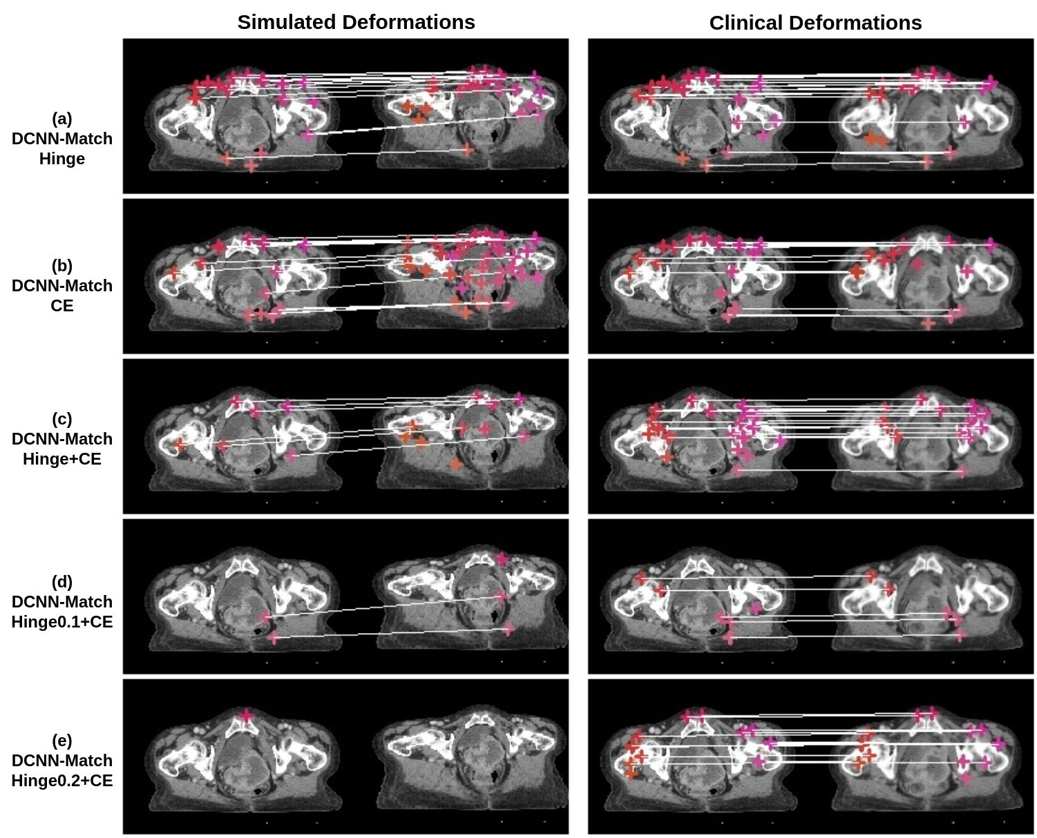
Fig 5: Visualization of predicted landmark correspondences by (a) DCNN-Match Hinge, (b) DCNN-Match CE, (c) DCNN-Match Hinge+CE, (d) DCNN-Match Hinge0.1+CE, and (e) DCNN- Match Hinge0.2+CE. A transverse slice from target and source CTs in the simulated deformations test set (left) and the clinical deformations test set (right) is shown. The corresponding landmarks are shown with the same colored cross-hairs in target and source image and a white line is drawn for in-slice corresponding landmarks. Please note that some corresponding landmarks may lie on a different slice and are therefore not visible in the figure.

3 Results

The average inference time of DCNN-Match variants for predicting landmark correspondences in one CT scan pair was ∼20s. A representative example of predicted landmark correspondences is shown in Figure 5. The images in the figure are shown with the couch table cropped for better visualization, but the automatic landmark correspondence detection as well as DIR were performed on full CT scans without any cropping.

25

Table 1: Number of predicted landmark correspondences per CT scan pair. Mean (M) ± standard deviation (SD), and range (5th percentile – 95th percentile) are provided.

193 – 1000

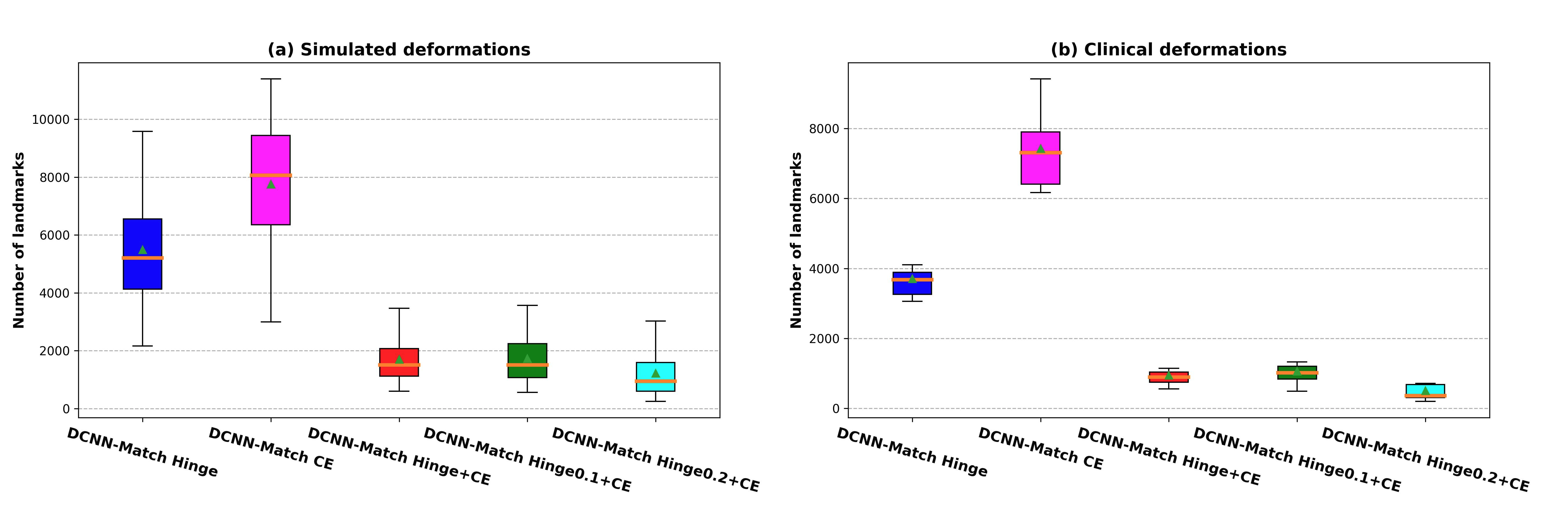
Fig 6: Distribution of predicted automatic landmark correspondences across patients. The boxes extend from the lower to upper quartile values of the data, with a line at the median. Mean is shown with a triangular marker and whiskers represent the range from 5th to 95th percentile.

3.1 Number Of Landmark Correspondences

The number of landmark correspondences predicted per image on the simulated test set and clinical test set is described in Table 1 and Figure 6. As can be seen in Table 1 and Figure 6, DCNN- Match Hinge and DCNN-Match CE approaches predicted a large number of landmarks per CT scan pair. In DCNN-Match Hinge+CE, the use of an auxiliary loss allows for applying an additional constraint on the landmark correspondences. Consequently, the number of predicted landmark

Match On The Simulated De-

formations test set - CT. correspondences per image was fewer than with using either of the loss separately. Further, the DCNN-Match Hinge0.1+CE and DCNN-Match Hinge0.2+CE predicted even fewer landmarks per CT scan pair, possibly due to the additional constraint posed by the positive margin mpos used in the Hinge loss. It should be noted that irrespective of the differences within different DCNN-Match variants, a considerable number of landmark correspondences were predicted by all of them in both the simulated as well as the clinical deformations test set.

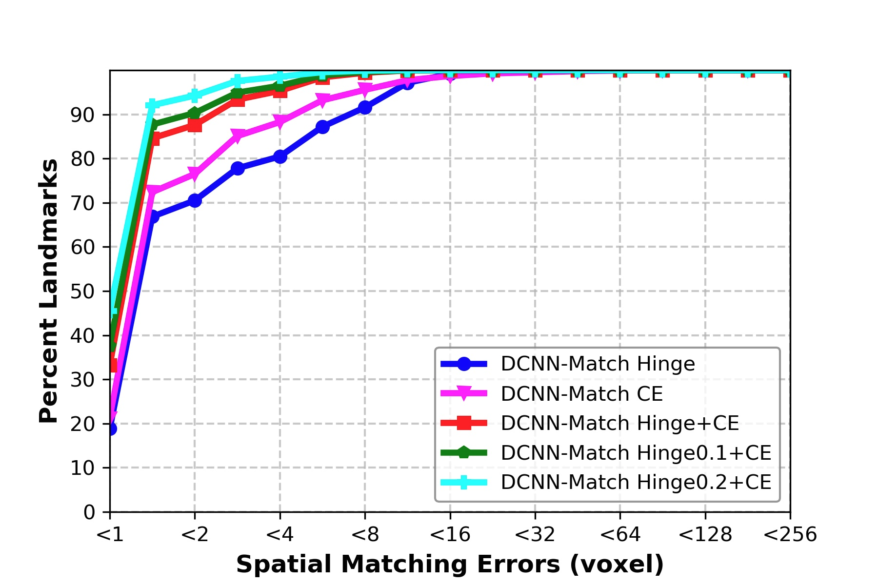
3.2 Spatial Matching Errors of Landmark Correspondences The cumulative distribution of the predicted landmark correspondences in the simulated test set is plotted against their spatial matching errors in Figure 7. Both DCNN-Match Hinge and DCNN- Match CE predicted more than 70% landmarks with less than 2 voxels (equivalent to 4 mm) spatial matching error. But, DCNN-Match CE predicted a higher percentage of landmarks within a spe- cific spatial matching error as compared to DCNN-Match Hinge. The decrease in spatial matching errors could be attributed to the added parameters used in the dedicated descriptor matching mod- ule in DCNN-Match CE as opposed to the parameter-free module in DCNN-Match Hinge. Fur-

27

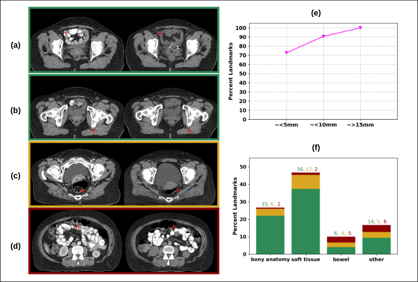
Fig 8: Validation of landmark correspondences in clinical deformations test set. Represen- tative examples of (a)-(b): good match despite contrast variation and difference in muscle defor- mation, (c): moderate match, and (d): wrong match. (e): Cumulative distribution of landmarks with respect to (approximate) spatial matching errors. (f): Distribution of landmarks in different anatomical categories. The bars are shaded in proportion to the number of landmarks correspond- ing to a rank: green = good, yellow = moderate, red = wrong. In each anatomical category, the total number of landmarks representing a rank is provided in the text above bars in the corresponding color.

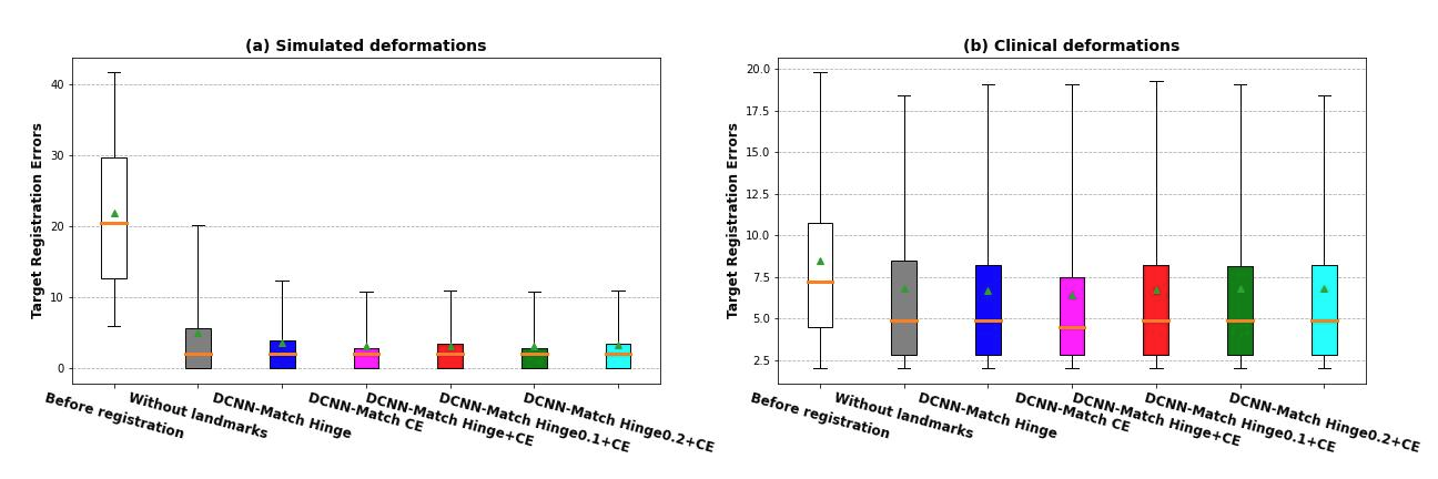
Fig 9: Distribution of Target Registration Errors (TRE). The boxes extend from the lower to upper quartile values of the data, with a line at the median. Mean is shown with a triangular marker and whiskers represent the range from 5th to 95th percentile.

28

ther, DCNN-Match Hinge+CE takes advantage of the auxiliary loss and therefore, the landmark correspondences are predicted with lower spatial matching errors. About 90% of the predicted landmarks had a spatial matching error of less than 4 mm.

As expected, training with mpos > 0 yielded landmarks with lower spatial matching errors as compared to DCNN-Match Hinge+CE (Figure 7). Specifically for DCNN-Match Hinge0.2+CE, more than 90% of the predicted landmark correspondences had spatial matching errors of less than 1 voxel, which is equivalent to 2 mm (image resolution). This finding indicates the potential of the automatic landmark correspondences predicted by the DCNN-Match variant for use in clinical applications.

3.3 Spatial Matching Errors In Clinical Data

In Figure 5, the predicted landmark correspondences from DCNN-Match variants on a represen- tative transverse slice from the clinical deformations test set are shown for the reader’s perusal. More examples are shown in Figure 8 (a)-(d). The border colors indicate the ranking given by the clinician: green = good, yellow = moderate, red = wrong match. Figure 8 (a) demonstrates a good match in the small bowel despite the difference of the underlying contrast and Figure 8 (b) demon- strates a good match in the muscle despite a change in the muscle deformation. In Figure 8 (c), both the landmarks are present in the rectum, but in different locations, although it was challenging to review because of the presence of the gas pocket and change in the muscle deformation. Fig- ure 8 (d) shows an example of a wrong match in the bowel. It is important to note the underlying challenges visible between the two scans in Figure 8 (d) e.g., difference in contrast, and content mismatch due to presence of gas pockets.

Figure 8 (e) shows that more than 72% landmark correspondences were ranked as good match

29

i.e., approximately within 5 mm distance and about 90% landmark correspondences were ranked to be within 10 mm distance. These results indicate only a small performance difference in com- parison to the simulated deformations test set (magenta curve in Figure 7 and Figure 8 (e)), which is expected due to the presence of additional challenges in the clinical data.

Further, in Figure 8 (f), the percentage of landmarks in bony anatomy, soft tissue, bowel, and other regions is plotted. The bars in the plot are shaded in green, yellow, and red colors in proportion to the ranking of the landmarks (green = good, yellow = moderate, red = wrong) in that anatomical category. It is worth noting that the wrong matches are mainly in the bowel region, where content mismatch may happen along with large deformations and intensity variations.

3.4 Effect Of Landmark Correspondences On Dir

In Table 2, the TRE values in the simulated and clinical deformations test sets are provided. In Figure 9, boxplots of TRE values are provided. In both test sets, there was a significant main effect of the experimental scenario (i.e., DIR without landmarks and with landmarks predicted by either one of the DCNN-Match variants) on the observed TREafter values, (χ(5) = 6620.117, p = 0e0) in the simulated test set and (χ(5) = 34.051, p = 0.000002) in the clinical test set. Note that in the simulated test set, the sample size was quite large (100 landmarks per scan × 121 scans = 12100) giving rise to near zero p values in the statistical testing.

In the simulated deformations test set, the post-hoc comparisons revealed that TREafter values from registration using additional guidance from landmark correspondences predicted by any of the DCNN-Match variants were significantly lower than TREafter values from registration without using additional guidance from landmark correspondences. However, the strongest effect was observed with landmark correspondences from DCNN-Match CE (p = 0e0).

30

On the clinical deformations test set, although the TREafter values from registration with the use of additional guidance by automatic landmark correspondences were smaller than the TREafter values from registration without using additional guidance from landmark correspon- dences, the differences were small. Only the post-hoc comparison between TREafter values from registration by using landmark correspondences predicted by DCNN-Match CE and TREafter val- ues from registration without using landmark correspondences yielded statistical significance after correction for multiple comparisons (p = 0.030).

Table 2: Target Registration Errors (TREs) in mm of pre-specified landmarks (for details refer to 2.7.2) before DIR but after affine registration (TREbefore) and after DIR with different approaches (TREafter). Mean (M) ± standard deviation (SD), and range (5th percentile – 95th percentile) are provided. Best TRE values are highlighted in bold.

∗Represents Significance In Post-Hoc

comparison against TREafter without landmarks.

Related Journal Articles & DOI Links

Selected peer-reviewed publications relevant to 12 Lead ECG Acquisition. Click the DOI to access the full paper (may require institutional access).

Why Choose Us?

Bangalore guidance for robotics, Spectre and autonomous systems projects.