Simulia Abaqus Aneurysm Wall

Wall modeling via function enrichment: extension to detached-eddy simulation Benjamin Krank, Martin Kronbichler, Wolfgang A. Wall∗

Abstract

We extend the approach of wall modeling via function enrichment to detached-eddy simulation. The wall model aims at using coarse cells in the near-wall region by modeling the velocity profile in the viscous sublayer and log-layer. However, unlike other wall models, the full Navier–Stokes equations are still discretely fulfilled, including the pressure gradient and convective term. This is achieved by enriching the elements of the high-order discontinuous Galerkin method with the law-of-the-wall. As a result, the Galerkin method can “choose” the optimal solution among the polynomial and enrichment shape functions. The detached-eddy simulation methodology provides a suitable turbulence model for the coarse near-wall cells. The approach is applied to wall- modeled LES of turbulent channel flow in a wide range of Reynolds numbers. Flow over periodic hills shows the superiority compared to an equilibrium wall model under separated flow conditions.

Keywords: Delayed detached-eddy simulation, Spalart–Allmaras model, Function enrichment, High-order discontinuous Galerkin

1. Introduction

Wall modeling via function enrichment is a spatial discretiza- tion technique that allows the resolution of the sharp bound- ary layer gradients present in high-Reynolds-number flows with relatively coarse meshes. The basic idea is to make use of the flexibility in Galerkin methods regarding the choice of the solu- tion space: a few additional, problem-tailored shape functions are used to approximate the solution, in addition to the common polynomials. Using these enriched elements, the full Navier– Stokes equations are solved in the whole boundary layer in a consistent manner. As a result, the wall model can take into account high adverse pressure gradients and convective effects, unlike most other wall modeling approaches.

The idea of wall modeling via function enrichment was pro- posed by Krank and Wall within the continuous Galerkin method (standard FEM) as a wall modeling technique for large- eddy simulation (LES). While that work showed promising re- sults in separated flows, the limiting factor in terms of accuracy was the turbulence model employed in the near-wall region.

A residual-based approach was used, supported by a structural LES model in the outer layer, a model that was originally not intended for underresolved boundary-layer simulations. The wall modeling approach was since applied in conjunction with RANS employing the Spalart–Allmaras (SA) model within the high-order discontinuous Galerkin (DG) method.

∗Corresponding author at: Institute for Computational Mechanics, Techni-

+49 89 28915300; Fax: +49 89 28915301

In this article, we show that the widely used delayed detached- eddy simulation (DDES) methodology may be used to model the unresolved turbulence in the near-wall region in wall mod- eling via function enrichment. This can be done by extending the implementation of the SA model in a straightforward way. The idea of the original DES approach is that the wall distance function y present in the SA model is limited with a

(1)

where the parameter CDES has been calibrated to CDES = 0.65 and the grid length scale is defined as the maximum of the cell length over the space dimensions ∆= max(∆x, ∆y, ∆z) . As a result, the RANS model acts as a one-equation LES subgrid model if y > CDES∆. DDES represents an enhancement of that methodology by defining the wall-distance parameter as

(4)

where u is the velocity vector, ν the kinematic and νt the eddy viscosity, and κ = 0.41. (D)DES is widely used in research and industry, see, e.g., [6, 7] and is today even used for the aerodynamics of entire vehicles due to its good accuracy in separated flows and the ability to investigate acoustic noise sources in the flow. Regarding the application of DES, two main branches are frequently used. The original idea was to simulate the whole boundary layer in RANS mode and to com- pute free shear layers in LES mode only . As an alternative,

December 25, 2017

arXiv:1712.08469v1 [physics.flu-dyn] 22 Dec 2017 DES can be seen as an approach to wall-modeled LES (WM- LES), in which only the inner layer is computed in RANS mode and the outer boundary layer in LES mode, see, e.g., .

Wall modeling via function enrichment has the potential of significantly reducing the computational cost of (D)DES. The grid saving of the standard (D)DES in comparison to LES is achieved by using relatively coarse meshes in the wall-parallel directions of up to 0.1δ (WMLES) and δ (classical DES) with the boundary layer thickness δ. The wall-normal direc- tion necessitates many grid points in order to resolve the lami- nar sublayer due to the requirement of placing the first off-wall

1 ∼1, However. For Example, If A Boundary Layer

of a thickness of 10,000 wall units is computed with a con- stant grid stretching factor of 1.15 , a total of 53 grid layers would be required. This is a quite high cost compared to the relatively low engineering interest in that region. Wall mod- eling via function enrichment allows the first grid point to be

1 ∼10 To 100, Saving 17–33 Grid Layers

for that example, without noteworthy loss in accuracy, in addi- tion to much better conditioned equation systems through the lower grid anisotropy.

In the next section, we give details on how the enrichment shape functions are constructed. In Section 3, the high-order DG code employed for the validation is outlined and numerical examples are presented in Section 4.

2. Wall Modeling Via Function Enrichment

The primary idea of wall modeling via function enrichment is as follows. In a single element row at the wall, the discrete ve- locity solution uh is composed of two parts, the standard poly- nomial component, ¯uh, and an additional enrichment compo-

Nent, Euh, Yielding

uh(x, t) = ¯uh(x, t) + euh(x, t).

(5)

The polynomial component is given in each cell as an FE-expansion

B Of Polynomial Degree K And Cor-

responding degrees of freedom ¯uB. There are several ways of constructing the enrichment component. In its simplest form, an enrichment function ψ is weighted in each element with one additional node eu0, i.e., one degree of freedom per space di-

Mension, With

euh(x, t) = ψ(x, t)eu0(t).

(7)

The enrichment function can additionally be weighted using a low-order polynomial to yield a higher level of flexibility in the function space [1, 2], which is not considered herein. It is this enrichment function that is responsible for the efficiency of the approach. By taking ψ as a wall function, the solution space of the Galerkin method is capable of resolving a sharp attached boundary layer with very few degrees of freedom. It is noted that this wall function is not prescribed as a solution, but the Galerkin method automatically “chooses” the best possible solution within the high-order polynomials and the enrichment component in a least squares sense. As a wall function, we

(8)

with κ = 0.41 and B = 5.17, as it was implemented in . Several alternative wall functions have been discussed in . In the wall-normal direction, Spalding’s law scales with the wall

Τw/Ρ And The Density Ρ Such

that the wall shear stress τw is represented correctly. In turn, the wall function has to be adapted according to the local wall shear stress in the numerical method, and its temporal evolution has to be taken into account.

We have developed an algorithm in [1, 2], which enables such an adaptation. Therein, the wall shear stress is computed on discrete nodes via the velocity derivative according to

B

of degree m = 1.

(10)

yielding a continuous representation of the wall shear stress. Through the choice of m = 1, the wall shear stress τw,h is a coarsened field, since usually k > 1; the coarsening is manda- tory because the wall functions are relations for the mean quan- tities, meaning that the mean wall shear stress is related to the mean velocity, and the average wall shear stress would other- wise be overpredicted, see Reference . This field is updated prior to each time step, such that the function space of the ve- locity changes continuously and adapts to the local flow con- ditions. Further details on the adaptation algorithm are given in . Near separation or reattachment locations, it may hap- pen that the wall shear stress becomes zero, which renders the function space linear dependent. However, considering that the first off-wall point is located very close to the wall in terms of y+ at these locations, a simple and consistent solution is to tempo- rally “switch off” the enrichment in the respective cells, see for details and for an evaluation of the method in WMLES in the context of another turbulence modeling approach. If wall shear stress becomes larger at these locations at a later instance, the enrichment is “switched on” again.

Finally, we comment on the two additional variables, which have to be discretized: the pressure and the working variable of the SA model. Both variables do not exhibit high gradients at the wall, such that they are represented sufficiently well by the standard FE space only, according to .

3. Numerical Method

The present wall modeling approach may be implemented in any FEM and DG flow solver. In this work, we consider the

2

implementation of the incompressible Navier–Stokes equations with the SA model in , which in turn is based on the incom- pressible high-performance high-order semi-explicit DG code INDEXA . An extension of the present wall modeling ap- proach to the compressible Navier–Stokes equations would be straightforward, since high gradients are commonly not present in the energy variable, such that the latter may be considered analogous to the pressure variable herein. Numerical methods based on the continuous FEM would require a small modifica- tion of the enrichment component as described in .

The solver is based on weak forms, which are described in detail in . These weak forms include volume and surface terms, that have to be integrated over cells and faces. The in- tegrals are in our solver evaluated using the high-performance kernels by Kronbichler and Kormann within the deal.II fi- nite element library . In particular, the integrals have poly- nomilal and nonpolynomial paths, the latter due to the nonpoly- nomial character of the enrichment function. The polynomial paths are integrated using the quadrature formulas given in and are evaluated exactly on affine cells. The nonpolynomial contributions have to be evaluated with more quadrature points, in particular in the wall-normal direction . From our exten- sive experience with wall modeling via function enrichment, we can give the following guide lines: If the enriched cells ex-

1E = 90 In The Statistical Quantities,

8 quadrature points in the wall-normal direction are sufficient.

Y+

1e = 200 (17 points); see also the monograph for further details. All simulation cases presented herein use an adaptive time stepping method presented in with a temporal accuracy of second order, a Courant number of Cr = 0.14, and a diffusion number of D = 0.02. In the particular formulation used with the enrichment, the solver has a formal spatial order of accuracy of k. Finally, we note that we apply no-slip boundary conditions weakly according to in all steps of the scheme for the ex- amples presented in this article, which limits the width of the first off-wall cell to a few hundred wall units, as the no-slip condition would otherwise be violated severely.

The increasing resolution power of the DG scheme with in- creasing polynomial degree should be taken into account in the (D)DES grid length scale ∆. Based on the analysis of the resolution power of DG schemes performed in , we choose

(11)

as a length scale, based on the respective cell size ∆e, in contrast to the choice of the factor of 1/k chosen in Reference .

4. Numerical Examples

Wall modeling via function enrichment is assessed by con- sidering DDES in the WMLES branch. In the first example, we investigate the method for attached equilibrium boundary layer flows present in turbulent channel flow. The second example considers flow over periodic hills in order to analyze the behav- ior of the enrichment in conjunction with DDES in a nonequi- librium flow. As a result of earlier studies [13, 19], the poly- Table 1: Overview of simulation cases for the turbulent channel flow. The number of polynomial grid points per direction i is Ni = (k + 1)Nie with the number of cells per direction Nie and the polynomial degree k = 4, ∆y+

1E Is The

thickness of the first off-wall cell, in which the enrichment is active, y = CDES∆ is the RANS–LES switching location in terms of channel half-height δ, and err(τw) is the relative error of the computed wall shear stress.

−1.4%

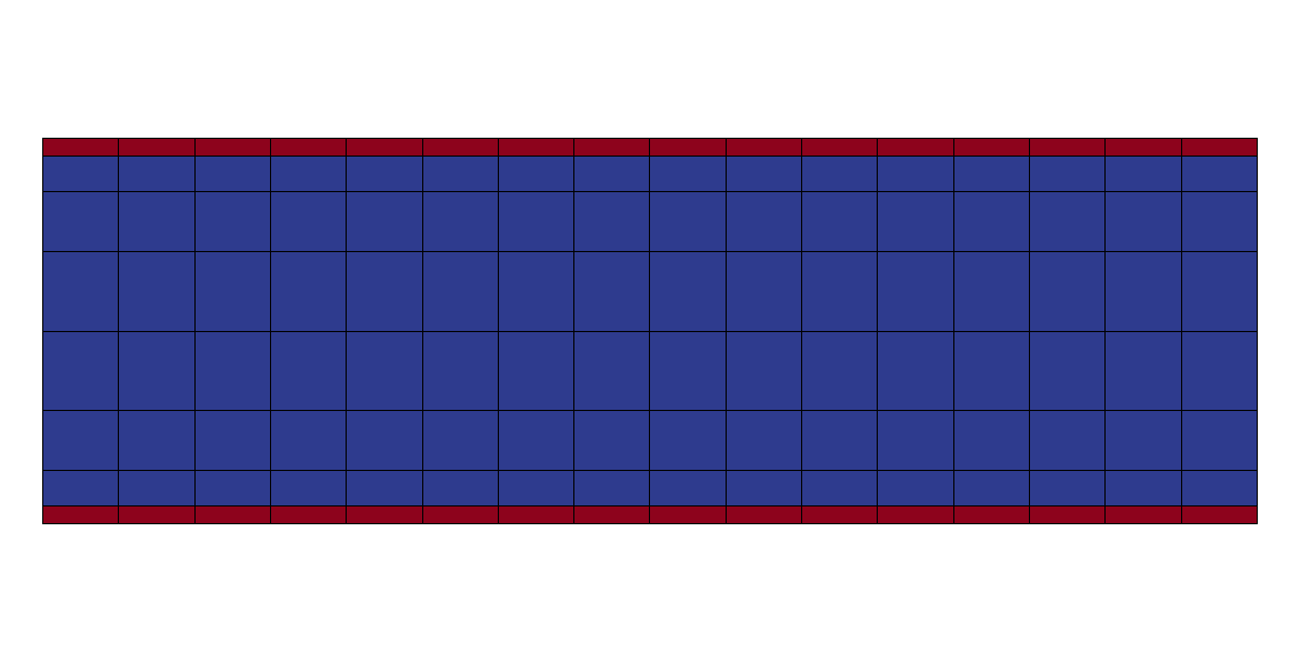
Figure 1: Mesh for turbulent channel flow at Reτ = 950. Red indicates enriched cells and blue standard polynomial cells, i.e., a single layer of cells at the wall is enriched. In each cell, the solution consists of a polynomial of 4th degree plus one enrichment shape function in the enriched cells.

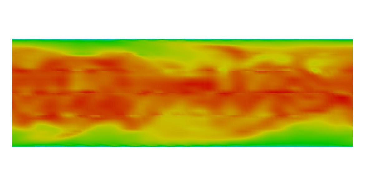
Figure 2: Instantaneous numerical solution of turbulent channel flow at Reτ = 950 via velocity magnitude. Red indicates high and blue low values. nomial degree of k = 4 has proven to be a good compromise between accuracy and time-to-solution, so this polynomial de- gree is used for all simulation cases presented.

4.1. Turbulent Channel Flow

We consider flow in a stream- and spanwise periodic chan- nel of the dimensions 2πδ×2δ×πδ in streamwise, wall-normal, and spanwise direction, respectively, with the channel half-height δ. The flow is driven by a constant body force, which is derived from the nominal quantities. We investigate this flow in a wide range of friction Reynolds numbers Reτ = uτδ/ν, which are chosen according to the available DNS data at Reτ = 395 ,

Reτ = 950 , Reτ = 2,000 , Reτ = 5,200 , And Ad-

ditionally Reτ = 10,000, Reτ = 20,000, and Reτ = 50,000. All simulation cases, meshes, and resolution criteria are presented in Table 1.

The meshes considered are chosen such that the wall-parallel

(U′V′)+

Figure 3: DDES (WMLES) of turbulent channel flow at several Reynolds numbers. Mean velocity (left) and RMS-velocities as well as Reynolds shear stress (right). All quantities are normalized according to u+ = ⟨u1⟩/uτ, u′+ =

3⟩/Uτ, And (U′V′)+ = ⟨U1U2⟩/U2

τ. grid length scale yields approximately ∆= 0.08δ for most cases, so the RANS–LES switching point is located at CDES∆= 0.05δ. One simulation case uses twice the number of grid cells in streamwise and spanwise direction, resulting in a RANS– LES switching point near CDES∆= 0.025δ. As for the wall- normal resolution, the enrichment is taken into account in the wall-nearest cell layer in all simulation cases, see Figure 1. As it was discussed earlier, the enrichment shape functions allow the resolution of the averaged near-wall flow with very coarse cell sizes. The width of the first off-wall cell lies in this work in the range of 51 to 191 wall units. In order to enable an applica- tion to high Reynolds numbers, a hyperbolic grid stretching is additionally considered, according to f: [0, 1] →[−δ, δ]:

(12)

with the mesh stretching parameter γ.

The Values Of Γ For

all simulation cases are included in Table 1. In the numerical method, the velocity solution is postprocessed at a large num- ber of wall-normal layers inside each cell using the definition of the velocity variable (5) such that the behavior of the enrich- ment may be analyzed. Statistics were acquired in a simulation time interval of approximately 60–95 flow-through times based on a fixed time interval.

The turbulent flow is visualized at one time instant in Fig- ure 2. Time-averaged results are presented in Figure 3. Therein, the results are plotted in terms of the normalized mean velocity

Τ, Which Are All Normalized Us-

ing the numerical value of uτ. The mean velocity is generally predicted very accurately in the laminar sublayer and the log- layer, where the enrichment shape functions are active. In or- der to get a better impression of the role of the enrichment, the numerical enrichment solution is plotted in Figure 3 alongside the full mean velocity solution. The enrichment solution repre- sents the largest part of the near-wall solution in most cases, including the high velocity gradient.

In Particular In Cases,

where the first off-wall cell spans a range of more than 100 wall units, the enrichment is the main contributor to the mean velocity. Solely at the lowest Reynolds number, the enrichment

Related Journal Articles & DOI Links

Selected peer-reviewed publications relevant to 12 Lead ECG Acquisition. Click the DOI to access the full paper (may require institutional access).

Why Choose Us?

Bangalore guidance for robotics, Spectre and autonomous systems projects.