Simulia Abaqus Cochlear Implant

Bimodal Cochlear Implants: Measurement Of The

Localization Performance as a Function of Device Latency

Difference

Rebecca C. Felsheim*+1,2, Sabine Hochmuth*3, Alina Kleinow1, Andreas Radeloff2,3,4, Mathias Dietz1,2

Oldenburg, Germany

2 Cluster of Excellence “Hearing4All”, Oldenburg, Germany

Abstract

Bimodal cochlear implant users show poor localization performance. One reason for this is a difference in the processing latency between the hearing aid and the cochlear implant side. It has been shown that reducing this latency difference acutely improves the localization performance of bimodal cochlear implant users. However, due to the frequency dependency of both the device latencies and the acoustic hearing ear, current frequency-independent latency adjustments cannot fully compensate for the differences, leaving open which latency adjustment is best. We therefore measured the localization performance of eleven bimodal cochlear implant users for multiple cochlear implant latencies. We confirm previous studies that adjusting the interaural latency improves localization in all eleven bimodal cochlear implant users. However, the latency that leads to the best localization performance for most subjects was not at the latency calculated to compensate for the interaural difference at intermediate frequencies (1 kHz). Nine of eleven subjects localized best with a cochlear implant latency that was slightly shorter than the calculated latency compensation.

Introduction

Binaural hearing, i.e., hearing with two ears, enables listeners to pinpoint the direction of a sound with remarkable accuracy. Trained normal hearing listeners can distinguish directions of two sources separated by angles as small as 1° in front of the head (Mills, 1958). In listeners with impaired hearing, the ability to localize sounds is reduced compared to normal hearing listeners. In a study by Dorman et al. (2016) which compared the localization performance of different subject groups, bilateral hearing aid users had an average root mean square error (RMSE) of 12° and bilateral cochlear implant (CI) users had an average RMSE of 29°. This stands against an average RMSE of 5° in an approximately age-matched normal hearing control group. An even larger average RMSE of 62°, close to chance performance, was reported in a small group of bimodal CI users with a hearing aid contralateral to the CI.

Most bimodal CI users used to be severely hearing impaired in both ears but were only eligible to receive one CI due to funding restrictions. With a high-power hearing aid, these patients receive some low-frequency hearing to complement their dominant CI, but, not surprisingly, they perform very poorly in sound localization, with little to no spectral overlap between CI and hearing aid stimulation. The bimodal participants in Dorman et al.

(2016) appear to fall into this category. However, when funding is less restrictive, a second very different group of bimodal CI users can be found: Those who have only a moderate hearing loss in one ear, that is best treated with a hearing aid, and a severe to profound hearing loss in the other ear, treated with a CI. These patients can already understand speech with their hearing aid alone and opt for the CI to get a more symmetric hearing sensation as well as to restore their spatial hearing. While better spatial hearing should be possible in this group due to a spectral overlap of both stimulation modalities, even this group has a rather poor sound localization with an average RMSE of 53° (Angermeier et al., 2021).

4

Multiple reasons are conceivable for the lower localization performance of the bimodal CI users. For instance, the human brain may not be able to integrate the two very different modalities of electrical and acoustic hearing well enough to enable binaural processing.

Other possible causes are the mismatches between the two ears caused by the two different devices and differently impaired ears. These include tonotopic mismatch, level mismatch, latency mismatch, and a mismatch in the spectral content between the two ears, caused by the CI not being able to selectively stimulate the apical turn and high- frequency limitation in the acoustic hearing ear (see Pieper et al., 2022 for a review).

The level mismatch has its roots in the often-independent fitting of the two devices and the reduced dynamic range especially in electric hearing. While it might be possible to balance the levels in the two devices for a specific stimulus, the reduced dynamic range makes it difficult to balance the levels for a wider range of stimuli.

The last dimension of mismatch is latency: In the acoustically stimulated ear, this latency consists first of the frequency and manufacturer-dependent processing latency of the hearing aid (1 - 7 ms; Zirn et al., 2015) and on the frequency and level-dependent latency of the human ear (1 - 8 ms; Ruggero & Temchin, 2007). For the CI side, only the latency of the device needs to be considered, which is frequency dependent and ranges from 0.5 - 7 ms for MED-EL CIs (Zirn et al., 2015), simulating the frequency dependency of the human ear, and a nearly frequency independent latency of about 12 ms for Cochlear devices (Engler et al., 2020). These different latencies add up to a latency mismatch of several milliseconds, vastly exceeding even the highest acoustically caused interaural time differences (ITDs) of about 740 µs (Hartmann & Macaulay, 2014), corresponding to a sound from 90°.

For bimodal MED-EL CI users, the latency on the CI side is lower than the combined latency (hearing aid latency + ear latency) on the acoustic side for all frequencies and hearing aid manufactures. Therefore, adding an additional delay to the CI processor is a promising option that is included in the most recent versions of the clinical fitting software Maestro since 2020. At present, only a frequency independent delay can be added. When

5

ear and device latencies are known or estimated, the presumed interaural latency mismatch can be derived. We call it “estimated latency mismatch”, and this value can be added to the CI processor.

Angermeier et al. (2021) measured the localization performance in bimodal MED-EL CI users with and without compensating for the estimated latency mismatch. They found that compensating for the estimated latency mismatch in bimodal patients acutely improved the localization performance significantly from an average RMSE of 53° to 38°. No further improvement was found after a familiarization period of three weeks Angermeier et al.

(2023). As the MED-EL CI latency is very similar to the latency of an acoustically stimulated ear, the estimated latency mismatch is approximately equal to the hearing aid latency, especially at frequencies near 1 kHz. At lower frequencies, the CI is a bit slower, and at higher frequencies even a bit faster (Zirn et al., 2015). Angermeier et al. (2021) therefore tested three different compensation delays: One that is equal to the hearing aid latency, 1 ms more, and 1 ms less. For 5 of 7 listeners, the lowest RMSE was obtained with the largest delay. Localization bias without added CI latency was always to the side of the CI and decreased as expected with increasing CI delay. But even for the largest delay, 6 of 7 listeners had a residual bias towards the CI. This may have been caused by mismatches in other dimensions, such as level (Pieper et al., 2022). We hypothesize that an even larger CI delay would compensate for the residual bias, possibly even further reducing the RMSE as well. A good compensation could possibly be able to reduce the RMSE to the range of bilateral CI users, as also hypothesized by Pieper et al. (2022). In this work, we have therefore measured the localization performance of eleven bimodal CI users with MED-EL CIs over a wider range of added CI latencies.

Estimated Latency Difference

Zirn et al. (2015) estimated the latency difference between the two ears based on measurements of the wave V of the auditory brainstem response. Following their approach, the latency on the acoustic hearing side is given as

(1)

with τHA(𝑓) being the potentially frequency-dependent latency of the hearing aid, τear(𝑓) the frequency dependent-latency of the ear and τ𝑉 the frequency-independent latency of the neural processing until wave V occurs. Similarly, for the electrically hearing side, the

(2)

where τCI(𝑓) is the frequency-dependent latency of the CI and τadd an additional latency that can be added to the processing latency. The value τ𝑉 is assumed to be the same for the acoustic and electric hearing side. The latency difference is then given as ∆𝜏 (𝑓) =  𝜏𝑎 (𝑓) − 𝜏𝑒(𝑓) = ( 𝜏HA(𝑓)  +  𝜏ear(𝑓) )  − (𝜏CI(𝑓)  +  𝜏add)

(3)

For MED-EL devices the difference between τear and τCI is very small. At 500 Hz τear is marginally smaller, at 1 kHz they are virtually identical and at 2 and 4 kHz τear is even a bit larger (Zirn et al., 2015). However, currently the clinical MED-EL software only allows for a frequency-independent additional latency. Therefore, a frequency-independent version of ∆𝜏(𝑓) needs to be estimated. We follow the approach of Angermeier et al. (2021) and assume an average equality between τear and τCI. This simplifies (3) to

(4)

as frequency-independent estimation of the latency difference between the two ears, with the frequency-independent estimate of the hearing aid latency τ̂HA.

7

For most participants, the hearing aid latencies (τ̂HA) were measured with the hearing aid analyzer unit ACAM 5 (Acousticon GmbH, Reinheim, Germany) using tone bursts in the frequency range of 500 to 4000 Hz. The hearing aid latency was measured from the time difference of the rising flank of the envelope between input and output. The median of the measured latencies in the frequency range of 500 to 4000Hz was taken as the general hearing aid latency. In a few cases (subjects S03, S04, and S06), the hearing aid latency was taken from the device delay list provided by MED‑EL1. The subject-specific hearing aid latencies are shown in Table 1. The hearing aid latency can be compensated for in the MED-EL CI fitting software Maestro starting from Version 9 for processors Sonnet 2 and Rondo 3 or newer.

Table 1: Subject-specific data of bimodal CI-listeners. Estimated hearing aid (HA) latency was generally measured with a hearing aid analyzer unit (median latency in the frequency range between 500 and 4000Hz). Latencies marked with an asterisk were taken from the ‘device delay list' provided by MED-EL. The everyday hearing aid latency compensation refers to the programmed hearing aid latency used in the subjects’ personal CI processors. “None” indicates that no HA latency compensation was used. Speech perception in quiet was measured at 65 dB SPL with a monosyllabic word test (Freiburg Monosyllables Test).

1 https://www.medel.pro/online-resources/timing-settings-for-hearing-aids

Participants

Participants were recruited from the clinical CI-center and all gave written informed consent. The study was approved by the local ethics committee (2020-022). The experiments were conducted in a sound-treated room at the CI-center.

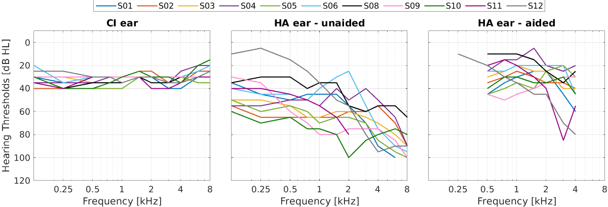
Eleven bimodal MED-EL CI listeners participated in the experiment. Their age ranged from 58 to 86 years. The listeners were fitted with a hearing aid contralaterally to the CI. Both devices were used daily. Unaided pure-tone averaged thresholds at 0.5, 1, 2, and 4 kHz (PTA4) on the hearing aid side ranged from 44 to 80 dB HL. Note that S11 had no measurable thresholds above 2 kHz. Therefore, a threshold of 120 dB HL was used for the PTA4 calculation at 4 kHz in this case. CI thresholds and both aided and unaided thresholds on the hearing aid side are shown in Figure 1.

Figure 1: Individual hearing thresholds with the cochlear implant (CI, left panel), unaided pure-tone thresholds contra- laterally to the implanted ear (middle panel) and aided thresholds with the hearing aid (HA, right panel) of all participants. Participants had at least four months of CI experience and achieved 50% or more correct responses with the Freiburg Monosyllables Test (speech perception in quiet) at a level of 65 dB SPL with each device, except for subject S02 and subject S09 who only achieved 25% and 35% correct with the hearing aid, respectively. Four CI users were already fitted with a hearing aid latency compensation  τadd =  τ̂HA on their personal processor. An overview of the subject-specific information is given in Table 1.

Experimental Setup

Sound source localization measurements were performed in a sound-treated room. The measurement setup consisted of 13 loudspeakers (8030C studio monitors, Genelec, Finland) placed in a semicircle with a radius of 1.35 m at ear height and 15° apart in the frontal azimuthal half-plane. Each stimulus consisted of three 70-ms long Gaussian broadband white noise bursts, each gated with a 5-ms Hanning window, separated by two 30-ms long silent intervals (similar to Angermeier et al., 2021). Each localization measurement consisted of 55 stimulus presentations (5 from each of the 11 most central loudspeakers). The presentations were randomized. Stimuli were presented at a level of 65 dB SPL. Random level roving of ±5dB was applied. Calibration was performed with a hand- held level meter (PCE-322A, PCE-Deutschland GmbH, Germany) at the subject’s head position.

All listeners used the same CI processor (MED-EL Sonnet2) during the measurements, which was programmed with the most frequently used individual map of each subject. All listeners, except for subject S04, used the FS4-processing strategy with four fine structure channels in their individual maps. Subject S04 used only three fine structure channels.

During testing, the adaptive intelligence program was disabled, and the microphone setting was set to “natural”. On the acoustic side, the listeners used their individual hearing aid with their everyday settings. Subject S11 had a slightly louder sound impression with the CI processor used for testing than with the personal processor, a Rondo3. Therefore, the CI-volume was reduced one step in the volume settings, which corresponded to a volume reduction of 4%. All other subjects performed the experiments at their average CI volume setting.

The global hearing aid latency compensation setting in the CI τadd was systematically varied for each measurement using the MED-EL fitting software Maestro 9. In general, six different latencies between 1.5 and 10 ms were applied (1.5ms, 2/3ms, 4/4.5ms, 6ms,

10

8ms, and 10 ms). Note that the software requires a minimal CI delay setting of 1.5 ms.2 If the everyday hearing aid compensation setting of a subject was close to one of the experimental latencies mentioned above, the everyday hearing aid compensation setting was used instead (e.g., subject S11 performed the localization experiment with a latency of 6.3 ms instead of 6 ms). In the case of subject S10 an additional measurement with an additional latency of 12 ms was conducted, since the hearing aid latency measurement using the hearing aid analyzer unit suggested a substantially higher latency in the lower frequencies (median of 11.3ms in the frequency range between 500 and 1000Hz) compared to the higher frequencies (median of 8.1ms). The first localization measurement was performed with the participants’ everyday hearing aid compensation setting (see Table 1 for individually used hearing aid compensation settings). The following localization measurements were conducted with randomized latency settings. In addition to the measurements with systematically varying latency settings, a retest measurement was performed at the end of the measurement session. Eight of the eleven subjects performed the retest, which was performed with the same latency setting as used for the first measurement. Four listeners did not perform all six planned latency measurements and retest due to technical problems (S01), fatigue (S04, S09) and pure monaural stimulus

Perception (S12)

2 The authors only became aware of the minimum latency of 1.5 ms to be set during the measurements. Therefore, the planned latencies were slightly adjusted after subject 08: 3 ms instead of 2 and 4.5 ms instead of 4.

12

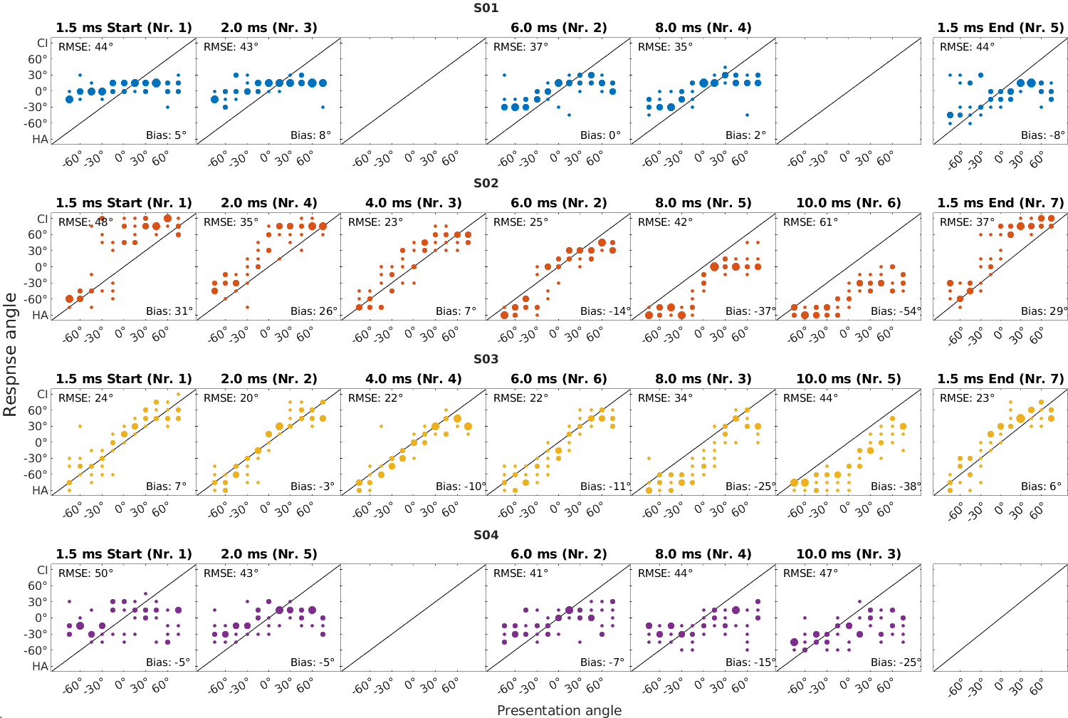
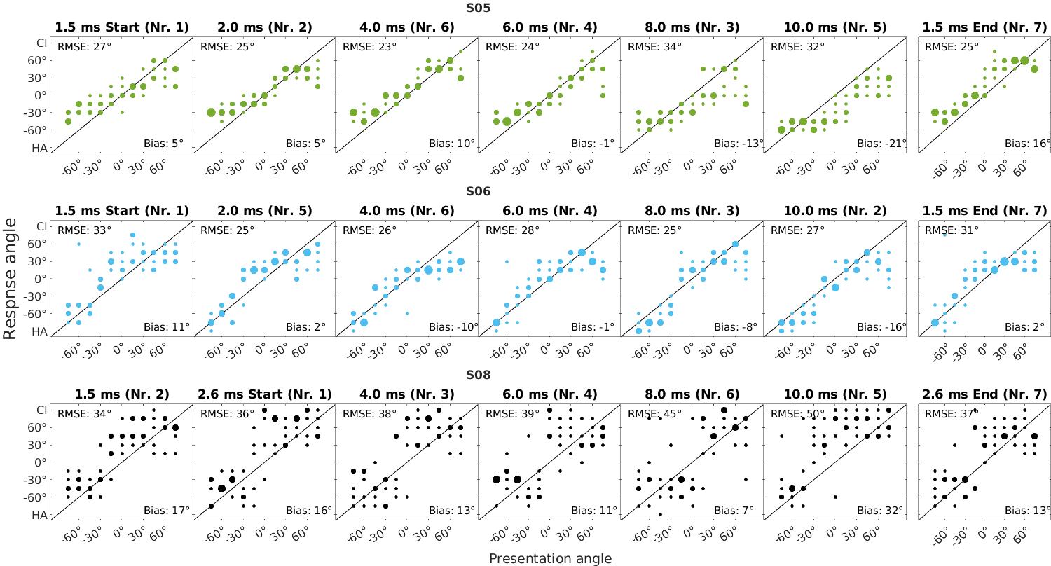
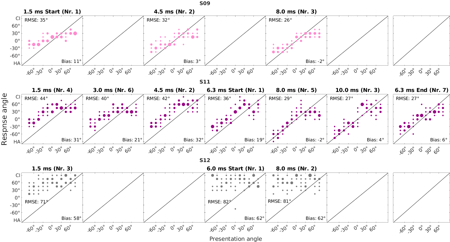
Figure 2: Bubble plots indicating the response angle over presentation angle for each subject and each of the additional CI latencies measured. Data was mirrored as needed, such that the hearing aid (HA) side is always at -90° and the CI side at +90°. The overall root mean square error (RMSE) and bias is shown in each subplot at the top left and bottom right corner, respectively. The number on top of each plot indicates the measurement order for the respective subject.

Results

On average, the root mean square error (RMSE) of the localization with the clinical settings was 39°, compared to 40° for Angermeier et al. (2023). When adjusting the latency settings to minimize the estimated latency mismatch, the mean RMSE improved marginally to 37°, compared to 32° for Angermeier et al. (2023). The mean of the lowest RMSE across all tested latencies was 32°.

Figure 2 shows the responded angle (y-axis) over presentation angle (x-axis), for each subject and each of the latencies added in the CI settings. Negative angles refer to the side of the hearing aid and positive angles to the side of the CI. Each dot indicates a response,

13

and larger dots are used to illustrate the same response for multiple repetitions of a presentation angle. If the active speaker was correctly identified the response would lie on the diagonal, which is illustrated by a line. At the top left of each panel, the RMSE for the current condition is given, and on the bottom right, the bias is depicted.

In cases with little or no added latency we expected a bias towards the CI. With increasing CI latency, we expected a shift in localization performance toward the center, combined with a decrease in RMSE, up to a subject-specific point. As latency was further increased, we expected an increasing bias towards the hearing aid side and again an increase in RMSE, since at some point the hearing aid side has a lower latency compared to the CI side. This pattern was observed in subjects S02, S03, S05 and S06. S03 had an overall lower bias compared to S02 and especially a lower bias towards the CI side. A similar pattern was shown by S10, and S11, although with more noisy responses. Both S05 and S11 tended not to use the full range of possible responses.

Subject S01 tended to localize everything towards the midline with very few responses to both sides. This became slightly less pronounced with increasing latency, but also with practice, as shown in the retest at the end. Similar responses were shown by S04 and S09, with a very noisy response pattern for S04, which did not become much clearer as the added latency was increased.

In contrast to the patterns above, S08 localized everything more to the sides. In the bubble plots themselves, it is difficult to see the influence of added latency, but when looking at the RMSE and bias a systematic effect can be seen. Subject S12 was completely unable to perform the task, as every stimulus was recognized from the CI side, and even there the loudspeaker selection was apparently random.

The first step in the data analysis was to evaluate the RMSE and bias for each condition and subject over the estimated latency difference (∆𝜏̂, Figure 3). A value of zero indicates an equalized latency between CI and hearing aid according to the estimated hearing aid latency. A negative estimated latency difference indicates that the hearing aid is faster

14

than the CI, and thus the CI is faster for positive values. To reduce the influence of the measurement noise, Figure 3 also shows quadratic fits for the RMSE and linear fits for the bias in the dashed lines in addition to the measured values. For the quadratic fits, we have constrained the x-axis shift to the range of the measured values.

We divided the subjects’ results into three groups based on their fitted RMSE and bias patterns and plotted them separately. Group 1 (first column in Figure 3) had the lowest fitted RMSE and the lowest fitted absolute bias for a positive estimated latency difference (or faster CI), implying that the estimated hearing aid latency was too long to achieve minimal RMSE and bias. This is the opposite to what Angermeier et al. (2021) reported. For all subjects in group 1, the RMSE shows the U-like shape we expected, with increasing error values as the estimated latency difference moves away from the optimum. This optimum, however, is not a clear minimal value, but multiple latency differences seem to result in a similar error.

Group 2 (second column in Figure 3) had the lowest RMSE and absolute bias for negative estimated latency differences (or faster hearing aid), implying that the estimated hearing aid latency was too short to achieve minimal RMSE and bias, as in Angermeier et al. (2021).

The RMSE of the subjects in group 2 just decreased with a higher added latency, and fitting a parabola in this data might seem a bit arbitrary. However, it is reasonable to assume that a further increase in the additional latency would cause the RMSE to increase again, as for group 1.

The bias values for both the groups 1 and 2 had a general tendency to move from the CI side (positive estimated difference) to the hearing aid side as the additional latency increased. For all subjects in these two groups, the bias was close to zero when the RMSE was minimal.

Related Journal Articles & DOI Links

Selected peer-reviewed publications relevant to 12 Lead ECG Acquisition. Click the DOI to access the full paper (may require institutional access).

Why Choose Us?

Bangalore guidance for robotics, Spectre and autonomous systems projects.