Simulia Abaqus Hip Contact

Andreas Burger1,2∗Luca Thiede1,2∗

Nikolaj Rønne3,4 Varinia Bernales1,5 Nandita Vijaykumar1 Tejs Vegge3,4 Arghya Bhowmik3,4 Alán Aspuru-Guzik1,2,5,6,7†

2Vector Institute For Artificial Intelligence

4CAPeX Pioneer Center for Accelerating P2X Materials Discovery

Abstract

Molecular Hessians, the second derivatives of the potential energy, are fundamental to many workflows in computational chemistry. Usually, accurate Hessians are computationally expensive to calculate and scale poorly with system size, whether computed using quantum chemistry methods or machine-learning interatomic potentials (MLIPs). In this work, we introduce Hessian interatomic potentials (HIPs), a deep learning model that directly predicts Hessians without relying on automatic differentiation or finite differences. To do so, we construct SE(3)- equivariant, symmetric Hessians from irreducible representation (irrep) features up to degree l=2, computed by a graph neural network. HIP Hessians are one to two orders of magnitude faster, more accurate, more memory efficient, easier to train, and exhibit more favourable scaling with system size. We validate our predictions across a wide range of downstream tasks, demonstrating consistently superior performance in transition state search, geometry optimization, zero-point energy corrections, and vibrational analysis. We open-source the HIP code and model weights.

Introduction

Molecular simulation is a cornerstone of material discovery and molecular design. While the pre- diction of energy and forces is often sufficient for structural dynamics, advanced computational chemistry workflows often depend on the molecular Hessian(Qu & Bowman, 2016; Huang et al., 2018). By describing the local curvature of the potential energy surface (PES), the Hessian is founda- tional to many computational workflows. Second-order geometry optimization relies on the curvature information to rapidly and reliably converge to equilibrium structuresSchlegel (2011). Transition state (TS) searches and extrema classification depend on the Hessian to correctly identify saddle points and reaction barriers, which are essential for parameterizing reaction rates and microkinetic models for longer time and length scale simulationsAndersen et al. (2019). Furthermore, mode-following Preprint.

Hip: Hessian Interatomic Potentials

transition state search methods directly leverage the curvature information to locate the transition statesHenkelman & Jónsson (1999). Finally, vibrational analysis uses Hessian eigenvalues to compute zero-point energy (ZPE) corrections and thermodynamic free energies bridging the gap from static molecules to non-zero temperature observablesGrimme (2012).

For a molecule with N atoms, the Hessian is a 3N × 3N matrix, where each entry requires a mixed second-order derivative of the electronic energy with respect to two nuclear coordinates. Despite their broad utility, Hessian calculations represent a substantial computational bottleneck.

Traditional approaches to obtain the Hessian rely either on analytic second derivatives or on numerical differentiation of gradients, both of which are very expensive, and analytical Hessians in particular are often so complicated to implement that they are not widely supported for all methods (Jørgensen & Simons, 1983; Handy & Schaefer, 1984; Komornicki & Fitzgerald, 1993).

Most computational chemistry calculations are carried out with Kohn-Sham density functional theory (Kohn & Sham, 1965) (DFT), due to its balance of computational cost and accuracy (Bursch et al., 2022). However, the O(N 4) scaling of hybrid DFT with system size remains expensive, which has spurred the development of machine-learning interatomic potentials (MLIPs). MLIPs promise to deliver near-DFT accuracy at a fraction of the cost while incorporating symmetries, thereby drastically reducing the need for extensive training data (Schütt et al., 2018; Thomas et al., 2018; Gasteiger et al., 2021; Schütt et al., 2021; Batatia et al., 2022; Batzner et al., 2022). While recent work demonstrates that automatic differentiation (AD) can successfully recover the Hessian (Yang et al., 2024; Yuan et al., 2024; Gönnheimer et al., 2025; Rodriguez et al., 2025; Williams et al., 2025; Cui et al., 2026), this approach faces two substantial limitations. High accuracy of the energy and forces does not guarantee comparably accurate second derivatives. Much like training on force labels is needed to achieve accurate force predictions Christensen & Von Lilienfeld (2020), explicit Hessian training labels are required for reliable AD Hessians (Zhao et al., 2025; Cui et al., 2026). Second, these AD Hessians introduce high computational costs, with an extra factor of ∼3N during training and inference (Yuan et al., 2024; Gönnheimer et al., 2025; Rodriguez et al., 2025; Williams et al., 2025; Cui et al., 2026). Rodriguez et al. Rodriguez et al. (2025) in particular showed that including the Hessian in the loss improves data efficiency and extrapolation of energy and force predictions but is limited by approximately 25 times longer training times, which make AD Hessians prohibitive to train. The same principle extends to learned exchange-correlation functionals, where supervising energy derivatives substantially improves accuracy (Eberhard et al., 2026). MLIPs can also be used to obtain Hessians with finite differences (Gönnheimer et al., 2025; Fu et al., 2025), an approach which requires less memory but 6N forward passes, and also requires specialized data collection schemes to be accurate Wander et al. (2025).

In this work, we introduce HIP: Hessian Interatomic Potentials. HIPs predict the Hessian directly, to eliminate the need for finite differences, coupled-perturbed equation solvers, or automatic differ- entiation. By building on SE(3)-equivariant neural networks, we demonstrate how HIP can predict Hessians at a fraction of the computational cost of traditional methods. A key observation is that one can construct the Hessian from spherical-harmonic features of the atom nodes and the messages between atoms, satisfying equivariance and symmetry constraints by design. In practice, HIP is not only faster but also more accurate than AD, enabling a variety of critical tasks in molecular

Simulations. Our Contributions Are The Following:

1. We present Hessian Interatomic Potentials (HIP), a method to construct SE(3)-equivariant, symmetric Hessians directly, without finite differences, coupled-perturbed solvers, or auto- matic differentiation, using an equivariant neural network backbone.

2. We show that downstream results can be improved further by using a loss function that

Targets The Relevant Hessian Subspace

3. We show that, compared to AD, the predicted Hessians are 10-100x faster, while also requiring 2-3x less peak memory on even small molecules with 5-30 atoms, with better saling.

4. We show that the predicted Hessians are more accurate on benchmark datasets, with 2x lower Hessian MAE, 3.5x lower eigenvalue MAE, and 1.5x higher eigenvector cosine similarity, and significantly better generalization to larger systems.

5. Finally, we validate the practical utility of our predicted Hessians in several downstream ap- plications, such as (i) zero-point energy corrections, (ii) second-order geometry optimization, (iii) transition state search, and (iv) frequency analysis for extrema classification.

Hip: Hessian Interatomic Potentials

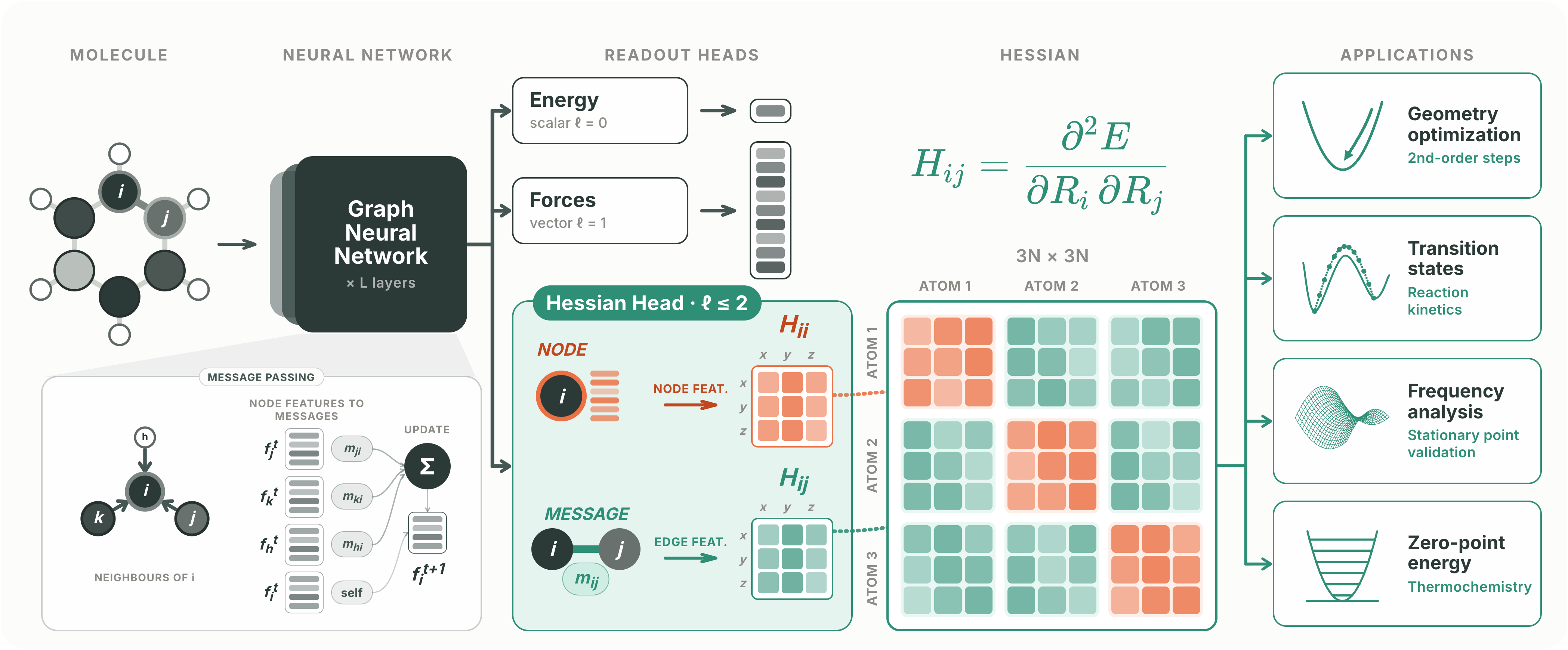
Figure 1: HIP architecture. A conventional MLIP (grey) maps a molecular geometry to its energy and forces. HIP adds an equivariant Hessian readout that combines node contributions (orange) and pairwise message contributions (green) to predict each Hessian block Hij = ∂2E/∂Ri∂Rj directly.

Conventional MLIPs instead construct the Hessian by automatic differentiation (AD) of the predicted energy or forces. The predicted Hessian supports geometry optimization, transition-state searches, frequency analysis and zero-point-energy calculations. HIP can use both direct force prediction and conservative forces.

Mlips And Equivariant Neural Networks

Early works on machine learning interatomic potentials used local atomic environment descriptors in combination with linear regression (Thompson et al., 2015; Shapeev, 2016), Gaussian processes (Bartók et al., 2010), and simple neural networks (Behler & Parrinello, 2007). SchNet (Schütt et al., 2018) was the first work to introduce rotation-invariant graph neural networks to predict molecular properties like energies and forces. Next-generation invariant architectures include ViSNet (Wang et al., 2024) and QuinNet (Wang et al., 2023). In parallel, rotation-equivariant architectures were developed, such as Cormorant (Anderson et al., 2019), DimeNet (Gasteiger et al., 2020), GemNet (Gasteiger et al., 2021), PaiNN (Schütt et al., 2021), NequIP (Batzner et al., 2022), SphereNet (Liu et al., 2022), MACE (Batatia et al., 2022) and the Equiformer family (Liao & Smidt, 2023; Liao et al., 2024). Graph neural networks represent a molecule as a graph G = (V, E) in 3D Euclidean space R3, with nodes/atoms I ∈V at positions rI ∈R3 and edges (I, J) ∈E defined by a cutoff radius. At layer t, each node carries a feature

I

that is a direct sum of irreducible SO(3) representations (irreps): h(t)

I,L,M}L

m=−l has 2l + 1 components. To update the node’s features, the model sends messages between each connected node, which are then aggregated in a permutation invariant fashion (usually the sum, or attention-weighted-sum operation) and then added to the receiving node. In SO(3)-equivariant GNNs, node features transform under a global rotation Q via Wigner D-matrices:

(1)

Translation equivariance is enforced by building messages from relative displacements rI,J = rJ −rI. If we want O(3) instead of SO(3) equivariance, each order-l feature has an extra parity label that determines the transformation under a global coordinate inversion.

Two irreps pl1 and gl2 interact using the Clebsch-Gordan tensor product (Thomas et al., 2018)

(2)

A message from source atom J to target atom I is then constructed as

Hip: Hessian Interatomic Potentials

where Yl2 is the 2l2+1 dimensional vector of the spherical harmonics of degree l2, wl1,l2,l3 : R →R is a learned weighting function, and fl1 a simple function that takes both node features in, for example concatenation in the case of EquiformerV2. A more efficient variation of equation 3 relying on the reduction of the SO(3) tensor product to the SO(2) tensor products was proposed by eSCN (Passaro & Zitnick, 2023) and adopted by subsequent works, such as EquiformerV2. Finally, the messages are pooled to update the node features, which can be done, for example, via a sum or using graph attention (Liao et al., 2024).

After several layers of message passing, task-dependent readout heads map the node features to the desired targets while respecting symmetry. For example, energies E are SO(3)-invariant per-graph scalars. The energy readout head therefore uses a global pooling and a reduction operation to output a l=0 feature. Forces F are SO(3) equivariant per-atom vectors (l = 1), and can be outputted either by a direct force readout head, or as the derivative of the energy F = −∇RE. As we will see in section 3, Hessians are SO(3)-equivariant per-graph matrices composed of per-atom-pair 3 × 3 equivariant sub-matrices.

Equivariant Matrix Prediction

There is a rich connection between the HIP Hessian prediction in this work and other rotation-equivariant matrices of interest, like Hamiltonian prediction Kaniselvan et al. (2025). For example, PhisNet Unke et al. (2021), QHNet Yu et al. (2023), HELM Kaniselvan et al. (2025), and WANet Li et al. (2025) predict the Fock matrix, and Graph2Mat Febrer et al. (2025) targets the density matrix.

Hessians From Dft

The gold standard for computing nuclear Hessians is to derive them analyti- cally. In Kohn-Sham DFT, this is achieved using the Coupled Perturbed Kohn-Sham (CPKS) method (Deglmann et al., 2002), which is employed to calculate the ground truth in the dataset and in the workflows of our experiments. If available, analytical Hessians provide the most efficient ab-initio way to obtain Hessians, but they still scale as O(N 5). See Appendix A.1.1 for details. A major downside of the CPKS approach to Hessians is its highly complex implementation and need for exchange-correlation-functional-specific derivations, which makes it not always available. An alter- native is to use a finite-difference scheme, requiring only energies or forces. Finite differences also scale O(N 5) for hybrid DFT, although with more numerical noise and a much larger computational prefactor. We provide more details in A.1.2.

Hessians From Mlips

MLIPs have gained widespread popularity for their ability to accurately approximate molecular energies and forces. The forces can either be directly predicted (Gasteiger et al., 2021; Liao et al., 2024), or calculated as the derivative of the MLIP energy using automatic differentiation. Previous work has shown that the Hessian can be calculated using AD to some success (Yang et al., 2024; Yuan et al., 2024; Gönnheimer et al., 2025; Rodriguez et al., 2025; Williams et al., 2025; Cui et al., 2026). Although AD Hessians are much cheaper to calculate compared to DFT, they still have some downsides. First, accurately modeling the energy does not guarantee low errors on Hessians (Yuan et al., 2024), but requires dedicated training (Zhao et al., 2025; Cui et al., 2026). Second, compared to energies and forces, Hessians are expensive: Given a probing vector v, AD only lets us calculate Hv. To calculate the full 3N × 3N Hessian, we need 3N Hessian vector products (HVPs) with the unit vectors v = ei, i = 0, ..., 3N −1, each yielding one column of the Hessian. Since the energy calculation with an MLIP is usually O(N), the total cost of the Hessian calculation is O(N 2). While the HVPs can theoretically be parallelized, the O(N 2) memory footprint requires even medium-sized systems to be computed sequentially. Rodriguez et al. (2025) in particular showed that including the Hessian in the loss leads to better extrapolation of energy and force predictions, less data for a given accuracy, and improved stability in MD. This comes at the cost of approximately 25 times longer training times, which makes AD Hessians prohibitive to train.

Rational Function Optimization (Rfo)

Geometry optimization locates minima arg minR E(R) of the potential energy surface (PES) starting from non-equilibrium molecular geometries. It underpins most workflows from global searches to high-throughput screening. If Hessians are available, second- order methods are favored due to their fast convergence guarantees (Nocedal & Wright, 2006; Doikov et al., 2023). RFO (Simons et al., 1983; Banerjee et al., 1985) is a commonly used second-order

Hip: Hessian Interatomic Potentials

optimizer (it makes use of Hessian information to accelerate convergence) for molecular geometries (Hermes et al., 2022). An attractive property of RFO is that it can be used both for minimizing E(R) as well as for finding saddle points, and it is robust to indefinite Hessians (Banerjee et al., 1985). As computing the Hessian is usually too expensive, a common practice is to maintain an approximate Hessian using the BFGS quasi-Newton scheme. We provide more details in A.2.

Zero-Point Energy (Zpe)

Zero-point corrections account for the quantum mechanical vibrational energy that molecules have at absolute zero temperature. To calculate the ZPE, one relaxes a geometry to an extremum, computes the Hessian, and sums the frequencies ZPE = ℏ

I

p˜λi. Here, ˜λi are eigenvalues of the mass-weighted Hessian ˜Hij = Hij/√mimj, and ℏis Planck’s reduced constant. One is usually interested in the relative ZPE between reactant and product states: ∆ZPE = ZPE(RP ) −ZPE(RR). The relative ZPE is relevant for reaction thermochemistry, as ∆ZPE enters as a correction to the reaction free energy ∆G and therefore the equilibrium constant, which relates forward and backward rates via detailed balance.

Transition States

Transition states (TS) are first-order saddle points on the PES. They represent the maximum barrier along the minimum energy path (MEP) between two minima. Identifying transition states is crucial for understanding reaction mechanisms and mapping reaction networks. A first-order saddle point is characterized by having exactly one negative eigenvalue of the Hessian. Over the years, various computational methods have been developed to describe MEPs and locate transition states. We review methods for transition state search in A.2.1.

To Carry Out Frequency Analysis, One Must First

remove the five or six redundant translational and rotational degrees of freedom, depending on whether the molecule is linear. This is done by mass-weighting the Hessian and performing an Eckart projection (Louck & Galbraith, 1976). Then, the projected matrix is decomposed into its eigenvalues, with all positive eigenvalues signaling a minimum, and exactly N negative eigenvalues signaling the presence of an order-N transition state.

Hip Hessian Prediction

Any equivariant neural network (Duval et al., 2024) with features of at least l = 2 can be equipped with a Hessian readout head. In this work, we use EquiformerV2 with four transformer layers as the backbone (Liao et al., 2024). Each layer contains a layer norm, message passing with graph attention, another layer norm, and a feed-forward layer. Rather than differentiating the scalar energy output, HIP adds a readout that constructs the full Hessian directly from the equivariant node features and interatomic messages. This makes the Hessian prediction parallel to the ordinary forward pass.

Hessian Symmetry Requirements

Hessians are symmetric, real-valued, Cartesian tensors. This means, under rotation of the coordinate system with rotation matrix Q, each Hessian sub-block HI,J transforms as

(4)

Any physically meaningful Hessian has to satisfy this rotation symmetry, as well as the symmetry of the upper and lower triangular H = H⊤. We elaborate on the symmetry of Hessians in A.3.

Hessian Prediction Head

Starting from T layers of message passing in the backbone, we use the atom features h(T )

I,M,C As Input

to a Hessian readout module. We first add a Hessian-readout-specific EquiformerV2 layer to improve expressivity. The Hessian is decomposed into 3 × 3 blocks HI,J, with diagonal blocks describing self-interactions and off-diagonal blocks describing pair interactions. Node features are used for the self-interaction terms, while messages between atoms I and J are retained as pair features rather than

Hip: Hessian Interatomic Potentials

By reusing the message-passing machinery with an interaction cutoff, the readout only constructs blocks for atom pairs within that cutoff. Its cost is initially O(N 2) for dense small systems but becomes O(N) for larger systems at fixed density, where the number of neighbors per atom remains bounded. The Hessian interaction cutoff can be set independently of the backbone radius to represent the locality of quantum-mechanical interactions. This sparsity-with-distance assumption aligns with the sparsity of Hessians due to the locality of electron interactions, which is common in quantum chemistry and can be mathematically rigorously justified (Kussmann et al., 2015). After message passing we have to transform the atom pair features hI,J,l,m,c into the corresponding Hessian sub- blocks HI,J. First, we project the pair feature irreps down to a single {˜hI,J,l,m}l∈{0,1,2} irreps feature (1x0e + 1x1e + 1x2e in e3nn notation (Geiger & Smidt, 2022)) using a linear layer Wl,c: ˜hI,J,l,m = Wl,chI,J,l,m,c We then expand ˜hI,J,l,m to an intermediate Hessian sub-block H′

Where Cl,M

l1,m1,l2,m2 are the Clebsch–Gordan coefficients ensuring that the relation in equation 4 is enforced (Unke et al., 2021). Physically, this is a simple change of basis from the coupled to the uncoupled angular momentum basis (Edmonds, 1996). H′

I,J,M1,M2 Is A 3 × 3 Block, Since M1 And

m2 run from −l1 = −l2 = −1 to l1 = l2 = 1. As Cl,m

L1=1,M1,L2=1,M2 = 0 For All L > 2, Hi,J,L,M,C

only needs to contain irreps up to l = 2 to build the 3 × 3 Hessian sub-blocks. Intuitively, equation 6 is the inverse of the irreducible tensor decomposition, so it assembles a spherical tensor back from its irreducible components. Conversely, this also means we need all irreps up to l = 2 as only including irreps up to l = 1 would not be sufficient to express the 3 × 3 tensors that decompose into l = 2 irreps. Finally, we symmetrize the intermediate Hessian to the final prediction with H = H′ + H′⊤.

Loss Function Design

To learn the Hessians, one can use standard loss functions like mean absolute error (MAE) or mean squared error (MSE) between predicted and actual Hessian elements:

(7)

However, we are often mainly interested in the smallest eigenvalues and the corresponding eigen- vectors (Besalú & Bofill, 1998; Cerjan & Miller, 1981). For this reason, we use a loss function that emphasizes the relevant subspace of the Hessian. This loss function is similar to Li et al. (2025), which uses it to emphasize the subspace up to the Lowest Unoccupied Molecular Orbital (LUMO) in Fock matrix prediction. Let V = [v1, v2, ..., v3N] be the matrix with columns made from eigen- vectors of the ground truth Hessian H, and Λ the corresponding matrix with eigenvalues on the diagonal and zeros everywhere else. Further denote V[:,:k] and V[:,k:] the matrices sliced to contain all columns up to/starting from the kth one. We can then define a subspace loss by

(8)

If Hpred = H we have V⊤HpredV = Λ, and the loss has therefore the correct minimum. Using L = LMAE/MSE + αLsub lets us emphasize the subspace corresponding to the k lowest eigenvectors and eigenvalues. Since the Hessian has five or six redundant translational and rotational degrees of freedom with eigenvalues close to zero, we need to set k > 6. In practice, we use k = 8. As we will show in A.5.1, predicting Hessians with HIP using any loss function significantly outperforms AD Hessians. MAE combined with the subspace loss in equation 8 further improves results in transition state search and extrema classification with frequency analysis by a small margin, which is why we use them in the experiment of the main text. For details and ablations of the choice of loss function see A.5.1.

Experiments

We evaluate our proposed approach for direct prediction of molecular Hessians across multiple tasks that test both accuracy and practical utility. Specifically, we measure prediction accuracy and quantify

Hip: Hessian Interatomic Potentials

computational speed-ups relative to AD and finite-difference Hessian calculation. We further assess downstream performance in geometry optimization, zero-point energy, and TS searches. For TS searches, we additionally perform frequency analyses to evaluate the reliability of the predicted Hessians in distinguishing true transition states.

Dataset And Training

We evaluate HIP on the Hessian dataset for Optimizing Reactive MLIP (HORM) (Cui et al., 2026), comprising 1,725,362 training geometries from Transition1x (T1x) (Schreiner et al., 2022), 50,844 T1x validation geometries, and 60,000 HORM-RGD1 geometries used for size-generalization tests.

All HORM energy, force, and Hessian labels were computed with GPU4PySCF v1.3.0 (Wu et al., 2025) using the ωB97X functional (Chai & Head-Gordon, 2008) and the 6-31G* basis set (Ditchfield et al., 1971; Hariharan & Pople, 1973), equivalently denoted 6-31G(d). Molecules are closed-shell neutrals with charge 0 and spin multiplicity 1. The self-consistent field was converged to an energy change below 10−10 Hartree and an orbital-gradient norm below 10−5, the GPU4PySCF v1.3.0 defaults. Analytical Hessians were obtained from the PySCF Hessian() implementation. Additional DFT calculations performed for this work use the same ωB97X/6-31G* level unless noted: PubChem size-extrapolation references with ORCA 6.0 (Neese, 2012) (A.6.7), glycine proton transfer with ORCA 6.1.1 at ωB97X-D3/6-31G(d) (A.6.6), and ReactBench DFT verification with GPU4PySCF v1.3.0 (A.6.3).

To isolate Hessian prediction quality from energy and force predictions, we train only the Hessian readout head while keeping the rest of EquiformerV2, pre-trained on energy, forces, and AD Hessians, frozen. This ensures that HIP-EquiformerV2 and AD-EquiformerV2 have identical energy and force predictions across all experiments. All AD-Hessian baseline models were trained on the same ground-truth DFT Hessians, so improvements are purely due to the advantage of HIP prediction over

Accuracy

We assess Hessian quality using the element-wise mean absolute error (MAE), the MAE of the eigenvalues λ and the smallest eigenvalue λ1, and the cosine similarity of the smallest eigenvector v1. We focus particularly on the lowest eigenvalue and eigenvector as they play an important role in downstream applications such as transition state search. We also measure the average inference time.

Table 1 shows results on the HORM-T1x validation set. The λ1 and v1 metrics are computed after mass-weighting and Eckart projection onto the vibrational subspace. Models trained only on energy and force labels, such as EquiformerV2 (E-F), have substantially higher Hessian errors, showing that accurate second derivatives require explicit Hessian training. Among the methods using automatic differentiation with Hessian training data, EquiformerV2 has the lowest errors. HIP-EquiformerV2 improves on all baselines across every reported metric. Compared with AD-EquiformerV2, HIP has 2.5× lower Hessian MAE, 3.8× lower eigenvalue MAE and higher eigenvector cosine similarity, while being 16× faster. End-to-end HIP training (marked by * in Table 1) reduces the errors further, reaching a Hessian MAE of 0.020 eV/Å2 at 31.4 ms per prediction.

Glycine Proton Transfer

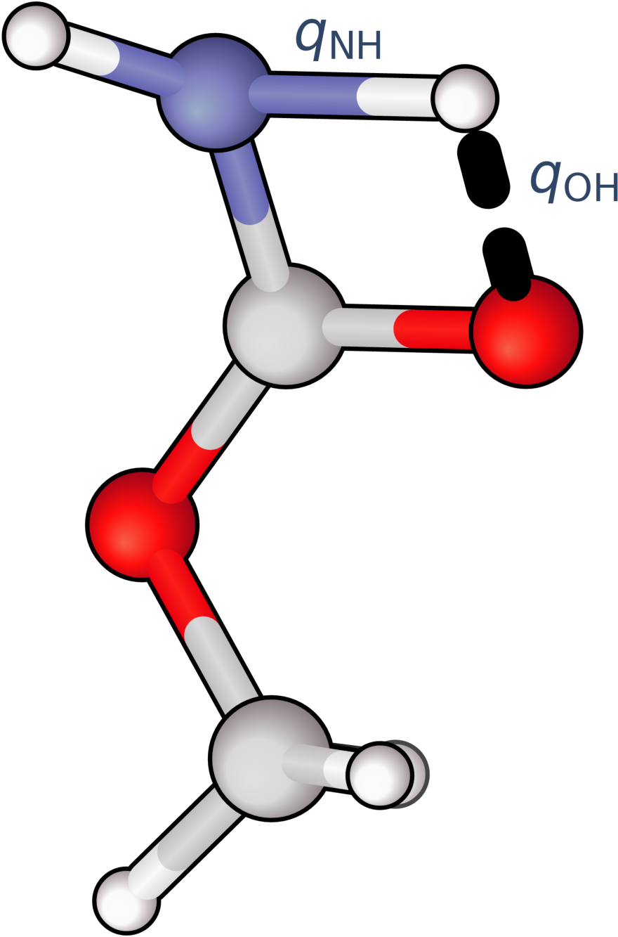
To assess Hessian quality along a chemically meaningful motion, we study the intramolecular proton transfer of glycine from the Transition1x test split Schreiner et al. (2022). We describe the transferring proton using its N–H and O–H distances, qNH and qOH, and define the proton-transfer coordinate ξ = qNH −qOH (see Sec. A.6.6).

We first study the two-dimensional (qNH, qOH) surface around the proton-transfer transition state. At each grid point, we place the proton at the target distances and relax all remaining degrees of freedom while keeping both distances constrained. The resulting geometries are then reoptimized at the DFT level. We characterize the surface by counting the negative eigenvalues (Fig. 2a). HIP closely reproduces the DFT topology, whereas AD introduces spurious negative modes near both the transition state and minima.

We next track the six lowest vibrational eigenvalues along a fixed, all-atom minimum-energy path as a function of ξ (Fig. 2b). HIP closely follows the DFT reference for all six modes. AD Hessians reproduce the lowest mode more closely but systematically underestimate the orthogonal curvatures

31.4

Table 1: Hessian prediction errors on the HORM-T1x validation set. Denoted are the mean absolute errors (MAE), cosine similarity (Cos), and average time per forward pass on an RTX 3060 GPU. λ1 and v1 were obtained after Eckart-projection. Bold values highlight the best-performing model. Baseline AD models are taken from Cui et al. (2026). In HIP-EquiformerV2 we trained only the Hessian readout head while keeping the parameters of the backbone frozen, while HIP- EquiformerV2* is trained end-to-end.

of modes 2–6. This agrees with Table 1, where HIP captures curvature information that AD Hessians miss. Finally, we project the Cartesian force F onto the unit tangent bξ of the minimum-energy path, F · bξ (Fig. 2c). We compare EquiformerV2 (EqV2) and LeftNet with conservative forces (LeftNet-CF), differentiating both models to obtain AD Hessians. Although both MLIPs reproduce the overall DFT force trend (left), their projected forces oscillate relative to DFT (middle). Differentiation amplifies these fluctuations into large Hessian errors along the path (right). Together with the spurious negative modes and underestimated orthogonal curvatures, this is consistent with AD Hessian errors arising from noise in the learned MLIP potential-energy surface.

Computational Efficiency And Scaling

A critical bottleneck in materials discovery is the scaling of compute with system size. Fig. 3a-b compares the inference time and memory footprint of HIP versus AD approaches. HIP exhibits the same scaling as a regular forward pass, with only a constant 25% additional time, roughly the cost of one extra layer on top of the four hidden layers. AD approaches, on the other hand, suffer from having to backpropagate through the graph for each row of the Hessian, which increases the cost to 3N of a forward pass. Quantitatively, HIP yields a 10× to 70× speedup on small molecules (5-30 atoms) and reduces peak memory usage by a factor of 2-3 compared to AD. This efficiency increases the size of systems for which Hessian-based workflows are computationally practical. AD calculations are also much harder to parallelize across a batch dimension; see A.4 for the explanation.

By comparison, since HIP reuses the message passing machinery, HIP parallelizes just as easily as the forward energy pass. We compared the batched AD Hessian as implemented by Cui et al. (Cui et al., 2026) with our HIP-EquiformerV2. At the largest evaluated HIP batch size, the per-sample inference time is at least 81× lower than that of their batch-one AD Hessian implementation; see A.4 for more details.

Generalization To Larger Systems

To assess extrapolation beyond the training distribution, we evaluate HIP on HORM-RGD1, using the published GPU4PySCF ωB97X/6-31G* labels, and on 710 PubChem samples containing 30–100 atoms (10 samples per atom count) (Kim et al., 2025), with reference Hessians computed with ORCA 6.0 at the same level (A.6.7). Fig. 3c-d shows the error of the Hessian eigenvalues as a function of the number of atoms, after mass-weighting and Eckart projection (A.6.7). We use the eigenvalues as a metric since their scale is independent of system size, while the MAE of Hessian elements lead to misleadingly low errors as a large share of Hessian elements go to zero for larger systems. HIP maintains strong performance across system sizes, with errors remaining relatively flat

Product

Figure 2: Glycine proton transfer. (a) Number of negative eigenvalues of the Eckart-projected, mass- weighted Hessian over the two-dimensional surface defined by the N–H and O–H distances, qNH and qOH. DFT is the reference; HIP is direct Hessian prediction; AD denotes Hessians differentiated from learned forces. Shading is the integer negative-mode count and black lines are DFT energy contours.

Circles, stars and triangles mark the reactant, transition state and product. In the rendering, carbon is grey, hydrogen white, nitrogen blue and oxygen red. (b) Six lowest Hessian eigenvalues along 145 minimum-energy-path (MEP) geometries versus ξ = qNH −qOH. DFT is shown as grey points, HIP as solid orange lines and EquiformerV2 (EqV2) AD as dotted blue lines. (c) Force projected onto the unit tangent bξ of the MEP (left), force residual relative to DFT (middle) and Hessian MAE (right).

DFT is shown as grey points, EqV2 AD as dotted blue lines and LeftNet-CF AD as solid purple lines.

Pubchem

Figure 3: Computational cost and molecular-size scaling. HIP is direct Hessian prediction; AD denotes Hessians differentiated from learned forces or energies; finite difference (FD) denotes numerical force differentiation. (a,b) Mean single-molecule inference time (a) and peak GPU memory (b) versus atom count on an RTX 3060 GPU; shading is one standard deviation over replicates. The forward pass is teal and dotted, HIP orange, direct-force AD blue, conservative-force AD purple and FD dark grey. The forward-pass and HIP curves overlap. (c,d) Mean eigenvalue MAE of the Eckart-projected Hessian versus atom count for HORM-RGD1 (c) and ten PubChem samples per atom count (d) (Kim et al., 2025); shading is one standard deviation over samples. HIP is shown by orange diamonds and AD by blue circles. The vertical grey dashed line in panel (c) marks the largest molecule size in the training set.

even for molecules larger than those in the training set. In contrast, the AD-based predictions show degraded performance along with the prohibitive computational costs for large molecules.

Geometry Optimization

We evaluate HIP Hessians in geometry optimization workflows, comparing exact second-order methods (rational function optimization, RFO) using Hessians against first-order methods and quasi- second-order RFO using BFGS. Fig. 4a shows convergence statistics across the validation set. RFO with HIP Hessians converges in the fewest steps on average, whereas finite-difference and AD Hessians often fail to converge within a 150-step budget. Naïve steepest descent rarely converges, underscoring the importance of curvature information. Wall-clock timings in Fig. 4a show the same trend. RFO with HIP Hessians is fastest overall because it requires fewer optimization steps and less expensive Hessian evaluations, whereas AD and finite-difference approaches are orders of magnitude slower.

Transition State Search

Transition state search is a central challenge in computational chemistry, requiring accurate Hessian eigenvalues and eigenvectors. We evaluate HIP using the ReactBench benchmark Zhao et al. (2025) with additional DFT verification (A.6.3). The workflow comprises four stages: the growing string method (GSM) first approaches the TS using energies and forces; RFO optimization with Hessians then refines the TS; the intrinsic reaction coordinate (IRC) then verifies connectivity; and a final DFT Hessian confirms the saddle point. Fig. 4b shows the success rates at each stage.

Zero-Point Energy

Figure 4: Downstream applications. HIP is direct Hessian prediction; AD denotes Hessians differentiated from learned forces; DFT is the reference. (a) Optimization steps and wall-clock time for 80 geometries. Violin shading is the sample distribution, points are individual geometries and crosses mark runs that did not converge within 150 steps. RFO wall-clock times with AD or finite-difference Hessians are omitted because they are one to two orders of magnitude longer than RFO with HIP. (b) Successful ReactBench samples after GSM, RFO, IRC, DFT transition-state verification and an additional tight force-convergence criterion, from 960 initial reactions (Zhao et al., 2025). DFT-verified full-set counts are extrapolated from fixed subsets of 100 TS proposals per Hessian method. (c) Mean absolute reactant ZPE error and reaction ∆ZPE error relative to DFT over 80 reactant–product pairs; the vertical axis is logarithmic. (d) Fraction of 1,000 stationary points for which the exact number of negative Hessian eigenvalues is predicted. Error bars in (c) and (d) are 95% bootstrap confidence intervals.

GSM performs equally well for both models because it relies only on energies and forces, which are identical. The differences emerge in Hessian-dependent stages. HIP achieves higher RFO convergence, better IRC verification, and most importantly, more DFT-verified transition states.

When requiring both DFT verification and tight convergence, HIP improves 12% over AD. These results demonstrate that HIP’s superior Hessian quality translates to more reliable TS identification, which is crucial for estimating reaction barriers and rates.

Zero-Point Energy

Zero-point energy is a critical thermochemical property derived from vibrational frequencies, which depend directly on Hessian eigenvalues. We evaluate both absolute ZPE at the reactant geometry and relative ∆ZPE between reactants and products (see A.6.4). Fig. 4c reveals dramatic improvements with HIP. For absolute ZPE, HIP achieves an order of magnitude better accuracy than LeftNet-DF and two orders of magnitude better than AD-EquiformerV2. For relative ∆ZPE, HIP similarly reduces the error by 97.03% compared to AD-EquiformerV2. These results demonstrate that HIP’s improved eigenvalue predictions translate directly to better thermochemical properties, where small errors in vibrational frequencies can lead to large errors in free energy.

Frequency Analysis For Extrema Classification

Characterizing stationary points on potential energy surfaces requires determining the number of negative Hessian eigenvalues: zero for minima, one for first-order transition states, and two or more for higher-index saddle points Maronsson et al. (2012). We test this capability on 1000 geometries from the HORM-T1x validation, comprising 44% first-order TSs, 37% minima, and 19% higher- order saddle points, as determined from DFT Hessians. Fig. 4d shows classification accuracy based

Number Of Atoms

Figure 5: Dataset scaling and force–Hessian error correlation. MAE is evaluated on the HORM- T1x validation set. (a–c) Energy (a), force (b) and Hessian (c) MAE versus the number of randomly selected training samples. EquiformerV2 trained on energies and forces is shown in dark grey; HIP trained end-to-end on energies, forces and Hessians is shown in orange. (d–f) Per-geometry force and Hessian MAE for 10,000 validation geometries using EquiformerV2 with Hessian supervision and AD Hessians (d), HIP trained end-to-end (e) and EquiformerV2 trained only on energies and forces with AD Hessians (f). Each point is one geometry. Colour indicates atom count. The displayed log-r is the Pearson correlation between the base-10 logarithms of the force and Hessian errors.

on counting negative eigenvalues. HIP achieves 92% accuracy, 10 percentage points better than the next-best AD model and 17 percentage points better than AD-EquiformerV2. This substantial improvement stems from HIP’s more accurate eigenvalue predictions, particularly for the small eigenvalues that determine the character of the stationary point. Accurate extrema classification is essential for automated reaction pathway discovery and for validating that optimizations have reached the intended type of stationary point.

Synergistic Improvements From Hessian Training

Thus far, we trained only the Hessian readout while freezing the backbone, isolating Hessian quality from energy and force predictions. We now investigate joint end-to-end training of the full model, including Hessian supervision. We train both the standard EquiformerV2 (energy and forces only) and the HIP-EquiformerV2 (energy, forces, and Hessians) for equal wall-clock time (3 days) across various dataset sizes. Fig. 5a-c reveals that Hessian supervision improves not only Hessian predictions but also energy and force accuracy across all data regimes.

On 10,000 validation structures (Fig. 5d-f), force and Hessian errors are positively correlated for Hessian-trained models, but nearly independent for an energy-force-only baseline, which can achieve good force accuracy while Hessian MAE remains an order of magnitude higher. HIP occupies a tighter, lower-error region than AD, indicating a more self-consistent potential energy surface.

This synergistic effect suggests that Hessian information provides a richer training signal, helping the model learn a better potential energy surface representation.

Non-Conservative Hessians

The practical implication of HIP is that second-order information can be used more routinely in computational workflows where its cost has previously been prohibitive. More broadly, expensive tensorial quantities with known symmetries may be represented by dedicated equivariant readouts, removing the need for costly differentiation of a learned scalar potential.

Hip: Hessian Interatomic Potentials

Direct prediction, however, does not guarantee that HIP Hessians are globally integrable or exactly consistent with the predicted energies and forces. Unlike non-conservative force errors, which can cause systematic energy drift during long molecular dynamics trajectories, Hessian errors in the applications considered here enter as local curvature estimates. This is consistent with the widespread use of approximate Broyden–Fletcher–Goldfarb–Shanno (BFGS) Hessians, which indicates that exact consistency is not necessary for all workflows (Appendix, A.3.1). Applications requiring exact energy–force–Hessian consistency may therefore need additional architectural or loss-based constraints.

Limitations

Other limitations are shared with existing MLIPs. Accuracy depends on the chemical and configurational coverage of the training data, and the finite interaction cutoff may omit long-range curvature contributions in ionic, polar or extended systems. Moreover, generating reference Hessians makes broad training coverage more expensive than for energy- and force-only models.

One possible way to reduce this data cost is to bootstrap HIP with approximate Hessian labels obtained by automatic differentiation of an energy-and-force model, followed by fine-tuning on a smaller set of reference DFT Hessians Gardner et al. (2024). The utility of such pseudo-label pre-training will depend on whether fine-tuning can correct systematic errors and noise in the initial AD Hessians, including the curvature errors observed here. Quantifying the trade-off between pseudo-label quality and the amount of reference Hessian data is therefore an important direction for future work.

Future experiments should validate HIP across broader chemical spaces and higher-fidelity electronic- structure methods. For periodic systems, the local construction can be adapted using a periodic neigh- bour list. The real-space supercell Hessian could then be Fourier transformed into the momentum- dependent dynamical matrix. The same symmetry-based, direct-prediction approach could also be extended to higher-rank response tensors. For example, the elastic tensor would require an additional global rank-4 readout containing l = 4 features, while predicting the cubic force constant tensor would require an atom-triplet rank-3 readout containing l = 1 and l = 3 features.

Conclusion

In this work, we have presented Hessian Interatomic Potentials (HIP), a method for directly predicting molecular Hessians using SE(3)-equivariant neural networks. Our approach eliminates the need for traditional computationally expensive methods, such as finite differences or automatic differentiation, offering a significant improvement in computational time, memory usage, and accuracy. Through extensive validation across a range of molecular tasks, we have shown that our predicted Hessians are highly effective for practical applications in computational chemistry.

Due to the versatility of the framework, any base model using spherical harmonics and message passing can be made HIP.

Author Contributions

Code, training, and experiments by A.Bu.; idea, theory, and Clebsch–Gordan transform code by L.T.; paper writing by L.T., A.Bu. and N.R.; visualizations by A.Bu. and L.T.; supervision and paper editing by N.R., A.Bh., T.V., V.B. and A.A.-G.; manuscript review by A.Bu., L.T., N.R., N.V., V.B., T.V., A.Bh. and A.A.-G.

Data And Code Availability

The HORM training and validation dataset is available from Zenodo at https://doi.org/10. 5281/zenodo.17217897 (Zhao & Han, 2025; Cui et al., 2026). HORM geometries originate from Transition1x (Schreiner et al., 2022), available from figshare at https://doi.org/10.6084/m9.

figshare.19614657.v4 (Schreiner, 2022). DFT calculations generated in this work, including atomic coordinates, energies, forces and Hessians for the PubChem CHNO size-extrapolation set, the glycine proton-transfer surface and the glycine minimum-energy path, together with trained HIP model weights, are available from Zenodo at https://doi.org/10.5281/zenodo.22003643 (Burger, 2026b) and from Hugging Face at https://huggingface.co/andreasburger/hip. The HIP source code is available at https://github.com/BurgerAndreas/hip under the Apache License, Version 2.0. A frozen snapshot is archived at Zenodo at https://doi.org/10.5281/

Hip: Hessian Interatomic Potentials

andreas-burger.com.

Acknowledgements

We are thankful for funding by the Pioneer Center for Accelerating P2X Materials Discovery (CAPeX), DNRF grant number P3. A.A.-G. thanks Anders G. Frøseth for his generous support. A.B. and L.T. acknowledge the AIST support to the Matter lab for the project titled "SIP project - Quantum Computing". A.B. is thankful for support through the Google NSERC IRC award. L.T.

thanks the NSERC for the support through the Discovery Grant. This research was undertaken thanks First Research Excellence Fund CFREF-2022-00042. Resources used in preparing this research were provided, in part, by the Province of Ontario, the Government of Canada through CIFAR, and companies sponsoring the Vector Institute.

Related Journal Articles & DOI Links

Selected peer-reviewed publications relevant to 12 Lead ECG Acquisition. Click the DOI to access the full paper (may require institutional access).

Why Choose Us?

Bangalore guidance for robotics, Spectre and autonomous systems projects.