Simulia Abaqus Spinal Implant

Implant Generation

Paul Friedrich1, Julia Wolleb1, Florentin Bieder1, Florian M. Thieringer1,2,

Basel, Switzerland

Abstract. Advances in 3D printing of biocompatible materials make patient-specific implants increasingly popular. The design of these im- plants is, however, still a tedious and largely manual process. Existing ap- proaches to automate implant generation are mainly based on 3D U-Net architectures on downsampled or patch-wise data, which can result in a loss of detail or contextual information. Following the recent success of Diffusion Probabilistic Models, we propose a novel approach for implant generation based on a combination of 3D point cloud diffusion models and voxelization networks. Due to the stochastic sampling process in our diffusion model, we can propose an ensemble of different implants per defect, from which the physicians can choose the most suitable one. We evaluate our method on the SkullBreak and SkullFix datasets, generating high-quality implants and achieving competitive evaluation scores. The project page can be found at https://pfriedri.github.io/pcdiff-implant-io.

Figure: System Model & Simulation Flow for Simulia Abaqus Spinal Implant

Keywords: Automatic Implant Generation · Diffusion Models · Point

Introduction

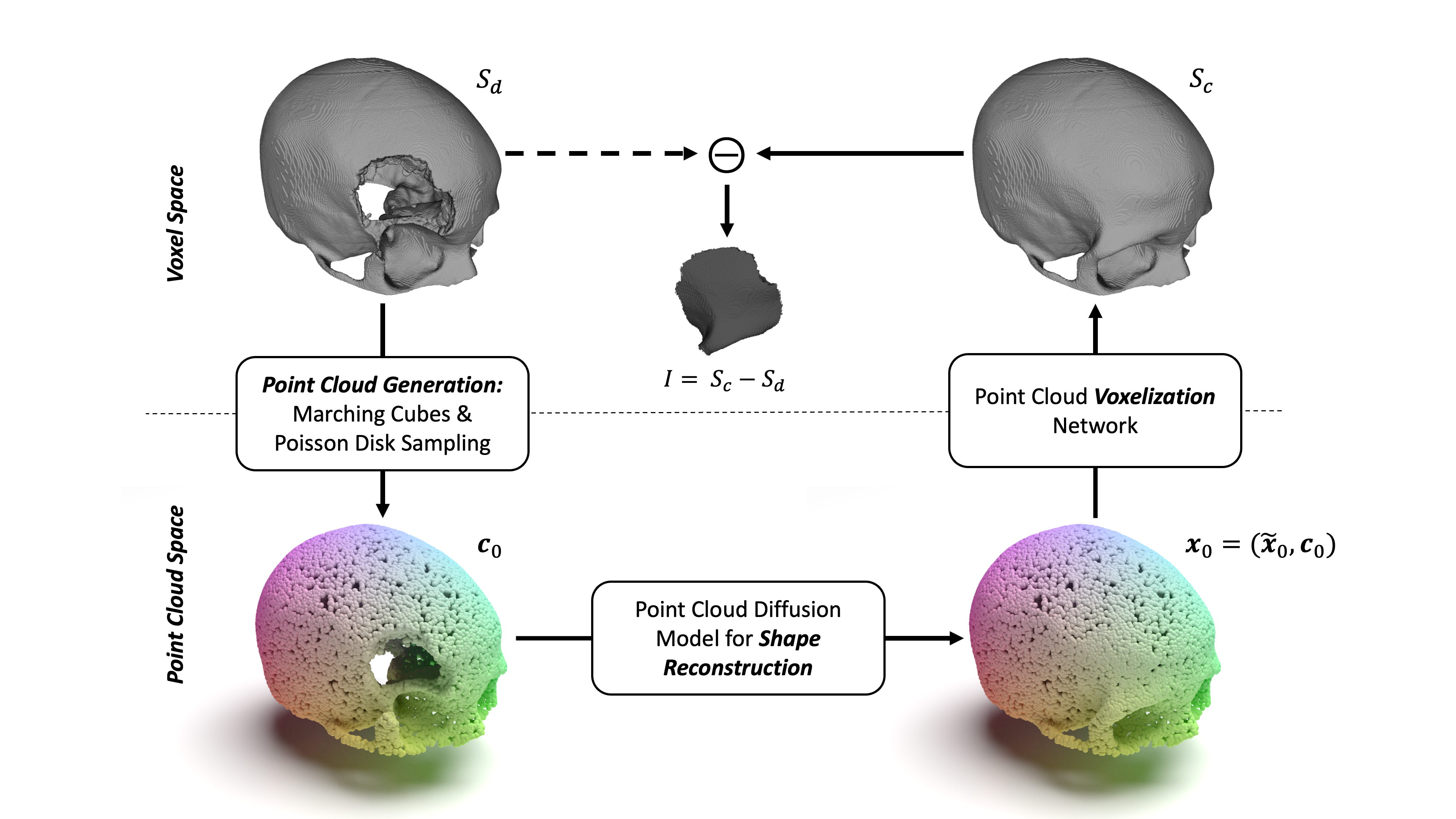
The design of 3D-printed patient-specific implants, commonly used in cranio- plasty and maxillofacial surgery, is a challenging and time-consuming task that is usually performed manually. To speed up the design process and enable point-of- care implant generation, approaches for automatically deriving suitable implant designs from medical images are needed. This paper presents a novel approach based on a Denoising Diffusion Probabilistic Model for 3D point clouds that reconstructs complete anatomical structures Sc from segmented CT images of subjects showing bone defects Sd. An overview of the proposed method is shown in Figure 1. Since performing the anatomy reconstruction task in a high reso- lution voxel space would be memory inefficient and computationally expensive, we propose a method that builds upon a sparse surface point cloud representa- tion of the input anatomy. This point cloud c0, which can be obtained from the defective segmentation mask Sd, serves as input to a Denoising Diffusion Proba- bilistic Model that, conditioned on this input c0, reconstructs the complete

2

P. Friedrich et al. Fig. 1. Proposed implant generation method with shape reconstruction in point cloud space. The implant geometry I is defined as the Boolean subtraction between completed output Sc and defective input Sd in voxel space.

Figure: System Model & Simulation Flow for Simulia Abaqus Spinal Implant

anatomy x0 by generating missing points ˜x0. The second network transforms the point cloud x0 back into voxel space using a Differentiable Poisson Solver . The final implant I is generated by the Boolean subtraction of the completed and defective anatomical structure. We thereby ensure a good fit at the junction between implant and skull. Our main contributions are: – We employ 3D point cloud diffusion models for an automatic patient-specific implant generation task. The stochastic sampling process of diffusion models allows for the generation of multiple anatomically reasonable implant designs per subject, from which physicians can choose the most suitable one.

Figure: System Model & Simulation Flow for Simulia Abaqus Spinal Implant

– We evaluate our method on the SkullBreak and SkullFix datasets, generating high-quality implants and achieving competitive evaluation scores. Related work Previous work on automatic implant generation methods mainly derived from the AutoImplant challenges at the 2020/21 MICCAI con- ferences. Most of the proposed methods were based on 2D slice-wise U-Nets and 3D U-Nets on downsampled or patch-wise data . Other approaches were based on Statistical Shape Models , Generative Adversarial Networks or Variational Autoencoders . This work is based on Diffu- sion Models , which achieved good results in 2D reconstruction tasks like image inpainting and were also already applied to 3D generative tasks like point cloud generation and point cloud completion . For retrieving a dense voxel representation of a point cloud, many approaches rely Point Cloud Diffusion Models for Automatic Implant Generation

3

on a combination of surface meshing and ray casting algorithms. Since surface meshing of unoriented point clouds with a non-uniform distribution is challenging and ray casting implies additional computational effort, we look at point cloud voxelization based on a Differentiable Poisson Solver .

Methods

As presented in Figure 1, we propose a multi-step approach for generating an implant I from a binary voxel representation Sd of a defective anatomical struc- ture.

Point Cloud Generation Since the proposed method for shape reconstruction works in the point cloud space, we first need to derive a point cloud c0 ∈RN×3 from Sd. We therefore create a surface mesh of Sd using Marching Cubes .

Then we sample N points from this surface mesh using Poisson Disk Sampling . During training, we generate the ground truth point cloud ˜x0 ∈RM×3 by sampling M points from the ground truth implant using the same approach.

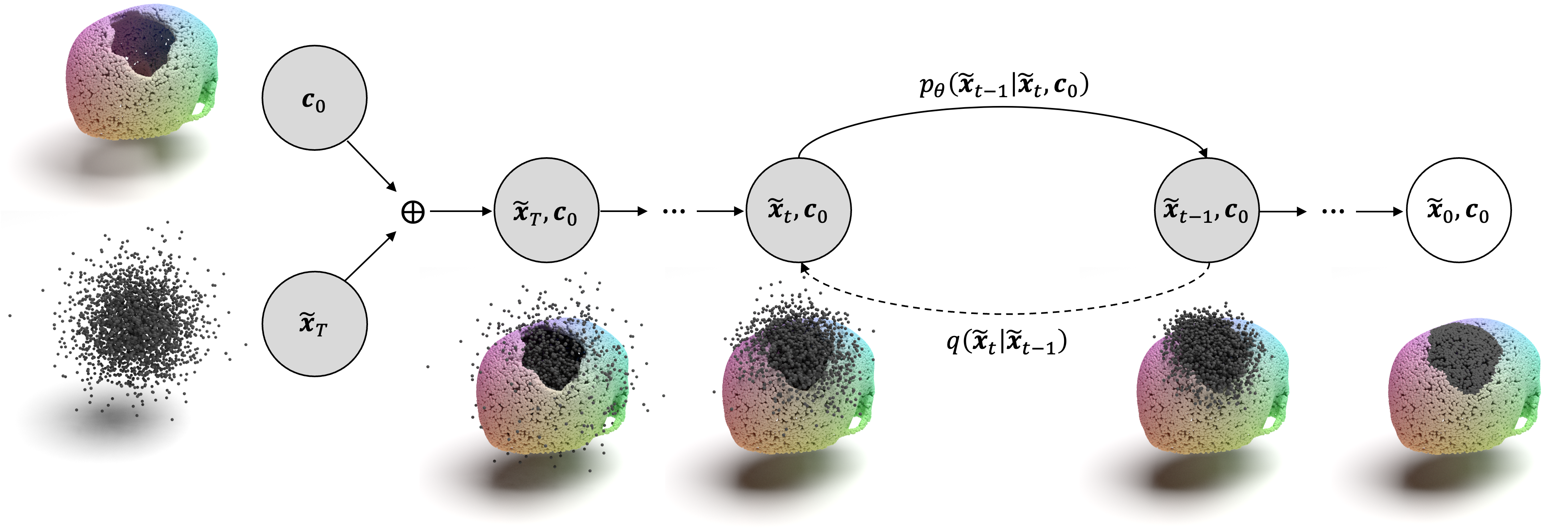
Diffusion Model for Shape Reconstruction Reconstructing the shape of an anatomical structure can be seen as a conditional generation process. We train a diffusion model ϵθ to reconstruct the point cloud x0 = (˜x0, c0) that describes the complete anatomical structure Sc. The generation process is conditioned on the points c0 belonging to the known defective anatomical structure Sd. An overview is given in Figure 2. For describing the diffusion model, we follow the formulations in . Starting from x0, we first define the forward diffusion process, that gradu- ally adds small amounts of noise to ˜x0, while keeping c0 unchanged and thus pro- duces a series of point clouds {x0 = (˜x0, c0), x1 = (˜x1, c0), ..., xT = (˜xT , c0)}.

This conditional forward diffusion process can be modeled as a Markov chain with a defined number of timesteps T and transfers ˜x0 into a noise distribution:

T=1

q(˜xt|˜xt−1).

(1)

Each transition is modeled as a parameterized Gaussian and follows a predefined variance schedule β1, ..., βT that controls the diffusion rate of the process:

P

1 −βt˜xt−1, βtI).

(2)

The goal of the diffusion model is to learn the reverse diffusion process that is able to gradually remove noise from ˜xT ∼N(0, I). This reverse process is also

4

P. Friedrich et al. Fig. 2. Conditional diffusion model for anatomy reconstruction in point cloud space. Points belonging to the defective anatomical structure c0 are shown in color and remain unchanged throughout the whole process. The forward and reverse diffusion processes therefore only affect the gray points ˜x0:T belonging to the implant.

with each transition being defined as a Gaussian, with the estimated mean µθ: pθ(˜xt−1|˜xt, c0) := N(µθ(˜xt, c0, t), βtI).

(4)

As derived in , the network ϵθ can be adapted to predict the noise ϵθ(˜xt, c0, t) to be removed from a noisy point cloud ˜xt. During training, we compute ˜xt at a random timestep t ∈{1, ..., T} and optimize a Mean Squared Error (MSE) loss

S=1 Αs. To Perform Shape Recon-

struction with the trained network, we start with a point cloud xT = (˜xT , c0) with ˜xT ∼N(0, I). This point cloud is then passed through the reverse diffusion

(6)

with z ∼N(0, I), for t = T, ..., 1. While this reverse diffusion process gradu- ally removes noise from ˜xT , the points belonging to the defective anatomical structure c0 remain unchanged. As proposed in , our network ϵθ is based on a PointNet++ architecture with Point-Voxel Convolutions . Details on the network architecture can be found in the supplementary material.

Voxelization To create an implant, the point cloud of the restored anatomy must be converted back to voxel space. We follow a learning-based pipeline proposed in . The pipeline shown in Figure 3 takes an unoriented point cloud x0 as input and learns to predict an upsampled, oriented point cloud ˆx with normal vectors ˆn. From this upsampled point cloud, an indicator grid ˆχ can be produced using a Differentiable Poisson Solver (DPSR). The complete voxel Point Cloud Diffusion Models for Automatic Implant Generation

5

Fig. 3. Voxelization pipeline based on a trainable network and a Differentiable Poisson Solver (DPSR). The trainable part learns to produce an upsampled point cloud ˆx with estimated normal vectors ˆn. The DPSR transforms (ˆx, ˆn) into an indicator function ˆχ from which a voxel representation can be derived.

representation Sc can then be obtained by evaluating the following equation for

0,

if ˆχ(i) > 0 .

(7)

During training, the ground truth indicator grid χ can be obtained directly from the ground truth voxel representation Sc and, as described in , is defined as:

−0.5,

if Sc(i) = 1 .

(8)

Due to the differentiability of the used Poisson solver, the networks can be trained with an MSE loss between the estimated and ground truth indicator grid: Lv = ∥ˆχ −χ∥2.

(9)

For further information on the used network architectures, we refer to . Implant Generation With the predicted complete anatomical structure Sc and the defective input structure Sd, an implant geometry I can be derived by

The Boolean Subtraction Between Sc And Sd:

I = Sc −Sd.

(10)

To further improve the implant quality and remove noise, we apply a median filter as well as binary opening to the generated implant. Ensembling As the proposed point cloud diffusion model features a stochastic generation process, we can sample multiple anatomically reasonable implant designs for each defect. This offers physicians the opportunity of selecting from various possible implants and allows the determination of a mean implant from a previously generated ensemble of n different implants. As presented in , the ensembling strategy can also be used to create voxel-wise variance over an ensemble. These variance maps highlight areas with high differences between multiple anatomically reasonable implants.

6

P. Friedrich et al.

Experiments

We evaluated our method on the publicly available parts of the SkullBreak and SkullFix datasets. For the point cloud diffusion model we chose a total num- ber of 30 720 points (N = 27 648, M = 3072), set T = 1000, followed a linear variance schedule between β0 = 10−4 and βT = 0.02, used the Adam optimizer with a learning rate of 2 × 10−4, a batch size of 8, and trained the network for 15 000 epochs. This took about 20 d/4 d for the SkullBreak/SkullFix dataset. For training the voxelization network, we used the Adam optimizer with a learning rate of 5 × 10−4, a batch size of 2 and trained the networks for 1300/500 epochs on the SkullBreak/SkullFix dataset. This took about 72 h/5 h. All experiments were performed on an NVIDIA A100 GPU using PyTorch as the framework.

SkullBreak/SkullFix Both datasets, SkullBreak and SkullFix , contain bi- nary segmentation masks of head CT images with artificially created skull de- fects. While the SkullFix dataset mainly features rectangular defect patterns with additional craniotomy drill holes, SkullBreak offers more diverse defect pat- terns. The SkullFix dataset was resampled to an isotropic voxel size of 0.45 mm, zero padded to a volume size of 512 × 512 × 512, and split into a training set with 75 and a test set with 25 volumes. The SkullBreak dataset already has an isotropic voxel size of 0.4 mm and a volume size of 512 × 512 × 512. We split the SkullBreak dataset into a training set with 430 and a test set with 140 vol- umes. All point clouds sampled from these datasets were normalized to a range between [−3, 3] in all spatial dimensions. The SkullBreak and SkullFix datasets were both adapted from the publicly available head CT dataset CQ500, which is licensed under a CC-BY-NC-SA 4.0 and End User License Agreement (EULA).

The SkullBreak and SkullFix datasets were adapted and published under the same licenses.

Results And Discussion

For evaluating our approach, we compared it to three methods from AutoIm- plant 2021 challenge: the winning 3D U-Net based approach , a 3D U-Net based approach with sparse convolutions and a slice-wise 2D U-Net approach . We also evaluated the mean implant produced by the proposed ensembling strategy (n = 5). The implant generation time ranges from ∼1000 s for Skull- Break (n = 1) to ∼1200 s for SkullFix (n = 5), with the diffusion model requiring most of this time. In Table 1, the Dice score (DSC), the 10 mm boundary DSC (bDSC), as well as the 95 percentile Hausdorff Distance (HD95) are presented as mean values over the respective test sets. Qualitative results of the different implant generation methods are shown in Figure 4 and Figure 5, as well as in the supplementary material. Implementation detail for the comparing methods, more detailed runtime information, as well as the used code can be found at https://github.com/pfriedri/pcdiff-implant.

Related Journal Articles & DOI Links

Selected peer-reviewed publications relevant to 12 Lead ECG Acquisition. Click the DOI to access the full paper (may require institutional access).

Why Choose Us?

Bangalore guidance for robotics, Spectre and autonomous systems projects.