Simulia Abaqus Wear Analysis

Creation and evolution of roughness on silica under unlubricated wear

Son Pham-Ba*, Jean-Franc¸Ois Molinari

Institute of Civil Engineering, Institute of Materials Science and Engineering, ´Ecole polytechnique f´ed´erale de Lausanne (EPFL), CH 1015 Lausanne, Switzerland Friction and wear are important phenomena occurring in all devices with moving parts. While their origin and the way they evolve over time are not fully understood, they are both intimately linked to surface roughness. Guided by pin-on-disc experiments, we present the steps giving rise to the formation of surface roughness on silica, first by the creation of roughly spherical wear particles whose size is related to a critical length scale governing the transition between ductile and brittle behavior, then by the accumulation of these small particles into a larger third body layer, or gouge. We show that, for the explored range of loading conditions, the surface roughness evolves toward a common steady state under unlubricated wear regardless of the initial surface roughness, hinting toward the possible predictability of roughness evolution in wearing components. The friction coefficient is shown to be related to the surface roughness and its time evolution is discussed as well.

Keywords: wear, friction, surface roughness, pin-on-disc, molecular dynamics, silica, third-body layer

1. Introduction

Friction coefficients and the way they evolve over time are currently hardly predictable. In order to better un- derstand friction, it is useful to relate it to known geo- metrical and physical characteristics of the tribological system. As the most simple friction laws suggest, like the Amontons-Coulomb’s friction law,1,2 friction forces are mostly independent of the apparent contact area, and are instead linked to the real contact area.3 Indeed, contacting rough surfaces only touch where protruding asperities meet, resulting in a real contact area being only a fraction of the total apparent contact area4–7 in most operating conditions. The ratio between real and apparent contact area is positively correlated with the normal load and is smaller for increasing surface roughness. Since frictional processes can only take place at the contact spots in an un- lubricated contact, this highlights a direct relation between friction and surface roughness. This relation applies to all engineered8,9 or natural surfaces,10 as they all display some roughness within a certain range of length scales.

Surface roughness itself can evolve thanks to wear. Molecular dynamics simulations of adhesive wear11 show that, at the nanoscale, two rough surfaces sliding on each other evolve toward fractal self-affine rough surfaces with the same fractal dimension regardless of the initial rough- ness. Another feature of these nanoscale simulations is the apparition of a rolling third-body particle, which seems to be a key factor behind the evolution of the surface rough- ness to self-affine characteristics.

At the engineering scale, experiments show that wear leads to the modification of the rubbed surfaces, with the formation of a third-body layer made of sintered worn material,12,13 also called tribo-layer14 or tribofilm,15,16 which contributes to a change in the frictional properties of the interface.

The same evolutionary behavior is found at the geo- logical scale. Gouge formation is omnipresent in brittle faults.17,18 It is made of crushed and worn rock particles and dictates the frictional properties of the interface, as

Seen Experimentally19–21 And Numerically.22,23

Studies also considered the evolution of surface rough- ness due to wear, for example in engineering applica- tions using pin-on-disc setups, where metallic samples can go through multiple wear regimes over time24 and settle down to a steady state after a certain amount of time. At steady state, the worn surfaces of the samples are seen to exhibit identical geometrical characteristics (wear track and surface roughness) regardless of the ini- tial surface roughness for the same operating conditions.25 Other studies reproducing or looking at geological phe- nomena observe a steady state self-affine roughness upon sliding after a running-in period.10,26–28 However, overall, the mechanisms of the onset of wear and their link with following wear processes are not studied in detail. A di- rect non-empirical relation between material properties and wear processes remains to be found.

Here, an experimental study of friction and wear was performed on amorphous silica (SiO2) using a rotating tribometer in a pin-on-disc configuration. From observa- tions of worn surfaces after various sliding distances, we deduced the steps giving rise to the creation of a sur- face roughness from comparatively flat initial surfaces — from the formation of the first third-body particles, often overlooked in the literature, to the full third-body layer — while attempting to directly relate the very first events of wear to material properties. The observations linked to the onset of wear are complemented by molecular dynamics (MD) simulations. We also assessed the evolution of the

Normal Load

Figure 1: Experimental setup on tribometer. The disc is fixed to a rotating motor. The ball can only move vertically and is kept against the disc with a constant normal load.

friction coefficient and of the surface roughness given dif- ferent initial surface roughnesses, and we provide a mech- anistic description of the factors behind surface roughness evolution.

2. Experimental Setup

The tribological tests have been performed using 6 mm spheres of amorphous SiO2 sliding (rotating) on discs made of the same material (see Figure 1). A Bruker UMT 3 tribometer was used. The sliding velocity of the ball was 8 mm/s and it followed a circular path of radius 1 mm with a normal load of FN = 1 N. Using Hertz contact theory, we get that in the elastic case the diameter of the contact zone between the unworn ball and the disc is 78.2 µm and the maximum pressure (reached at the center of the contact zone) is 312 MPa (see Appendix A.1).

The initial untreated surface roughness of the balls and the discs has been identified using atomic force mi-

Croscopy (Afm) And Is Around Sa ≈10 Nm, Which Is

very small from an engineering point of view (see Ap- pendix A.2 for details about the computation of the Sa surface roughness). Some discs have been manually pol- ished using P120 and P80 sandpaper, resulting in rough- ened surfaces with Sa = 0.74 µm and Sa = 1.41 µm in average respectively (computed from topographic images of size 117 µm × 88 µm and resolution 1360 px × 1024 px obtained on a Sensofar S-Neox confocal microscope). Only the discs were treated to have an initial surface roughness, while the balls were kept flat, with their initial roughness of Sa ≈10 nm. It is indeed difficult to polish the SiO2 balls in the same way as the discs without disrupting their spherical shape. Shot peening or sandblasting could have been used to roughen the balls, but having them initially smooth is not very important for this study since a surface roughness (dissimilar to the one on the discs) eventually develops on them.

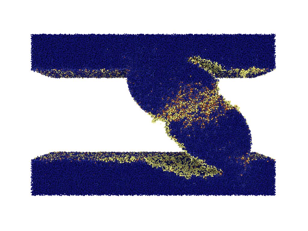
Table 1 lists the tests that were performed. The initial Sa of the discs are indicated. Some variation in the Sa roughnesses can be seen amongst the discs which were polished with the same grain size. This is in part due to the inherent variability of the manual polishing process.

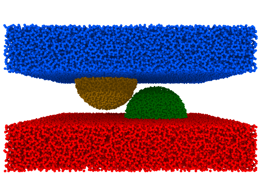
Table 1: Duration and initial roughness of the tests. The table is subdivided into three sections according to the polishing of the discs. The latter are manually polished using sandpaper with the indicated grain sizes. Each test has a duration and a corre- sponding sliding distance, known from the fixed sliding velocity of 8 mm/s. The third column indicates the number of repetitions for each set of parameters, and the multiple initial disc Sa are indicated for each repetition when they differ significantly.

Distance

Rep.

1.58

The fact that those roughness measurements were only performed in a single small window on each disc can also imply some uncertainty.

For each test, the Sa roughness of the disc is measured before and after the experiment (details in Appendix A.2). The vertical reaction force Fz and the lateral force Fx par- allel to the direction of sliding are recorded during the whole test, from which a dynamical friction coefficient µ = Fx/Fz is deduced. Roughness measurements cannot be similarly performed over the whole duration of a test because they are not in situ measurements. Finally, scan- ning electron microscope (SEM) images of the wear tracks and wear particles formed on the initially flat discs were taken after various durations.

3.1. Initial Wear Particle Size

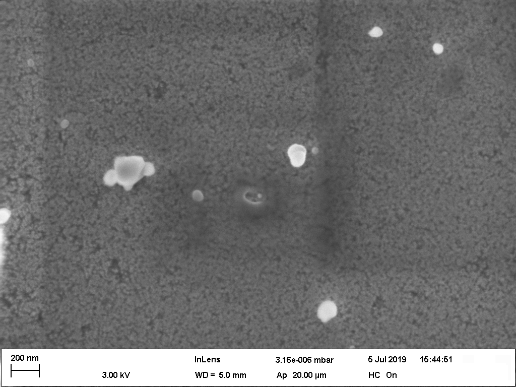
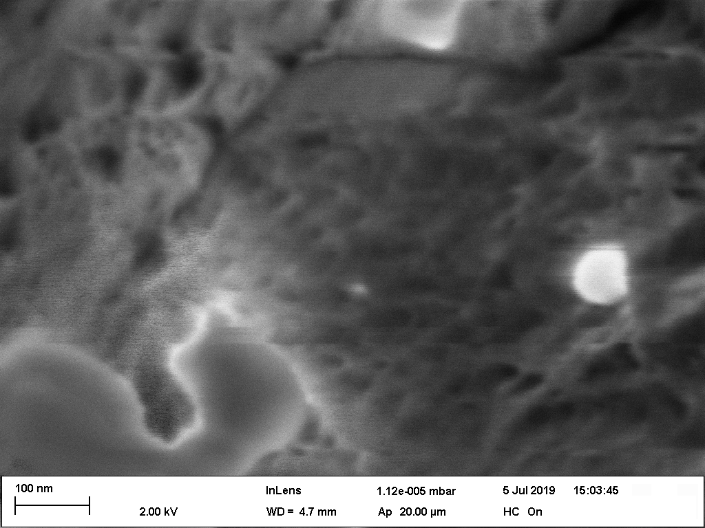
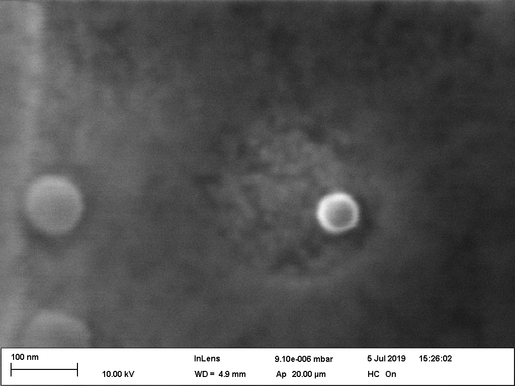
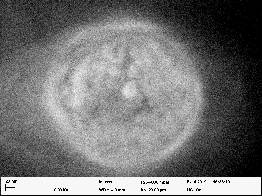
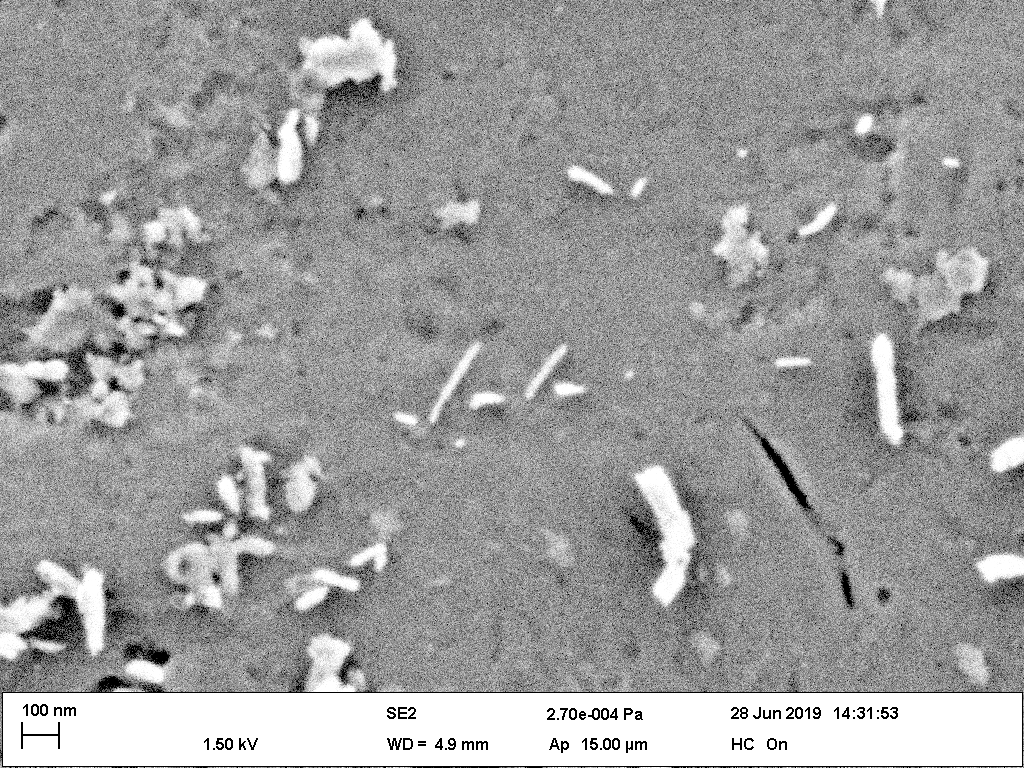
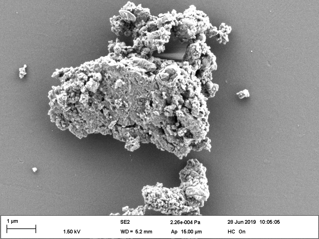
Figure 2 shows SEM images of wear particles found on a flat disc after only 1 s of sliding, corresponding to a sliding distance of 8 mm. The images were obtained using a Zeiss SUPRA 55-VP SEM. The formation of wear particles is the first and only evidence of wear found on the disc at this stage (there is no wear track). An adhesive nickel patch was rubbed against the surface of the worn disc to capture the wear particles in order to more easily observe them with SEM. No particle smaller than 30 nm was observed.

Whether this size depends on the material properties or the loading conditions is discussed thereafter.

32 Nm

(d) The silica was discriminated from the nickel background using

Energy-Dispersive X-Ray (Edx) Spectroscopy

Figure 2: SEM images of wear particles taken from a flat disc after 1 s (8 mm) of sliding. The particles were collected from the disc using an adhesive nickel patch for an easier observation. Recent theoretical work29 has confirmed the existence of a critical length scale d∗which governs a transition be- tween ductile and brittle behavior for any given material.

The expression of d∗for the detachment of spherical wear

(1)

where γ is the surface energy of the material, G is the shear modulus and σj is the shear strength (or flow stress) of cold welded junctions. Note that d∗is mainly dependent on ma- terial parameters and weakly depends on geometry and loading conditions (which influence the ‘12’ factor), thus it can be itself considered as a material parameter. A sheared junction between two surfaces can only be detached into a wear particle if its size d is larger than d∗. Otherwise, it flows plastically. It implies that no wear particles smaller than d∗should be observed in wear experiments, because they cannot be created.

Using MD simulations, we computed estimates for the unknown material parameters of amorphous SiO2 using a potential by Vashishta et al.30 taking into account three- body interactions, using a cutoff parameter of rc = 8 ˚A.

The amorphous SiO2 MD system is prepared following the procedure of Luo et al.,31 starting from a β-crystobalite structure. The system is heated and cooled by equilibrat- ing it for 90000 timesteps of 0.5 fs at 5000, 4000, 3000, 2500, 2000, 1500, 1000, 500 and 300 K, with cooling periods with a rate of 166 K/ps between each constant temperature step, except when going to 300 K where a rate of 13 K/ps is used. The pressure is always kept at 0 using a Berendsen barostat. The isotropic material properties of the obtained material at 0 K are E = 120 GPa, ν = 0.22 and G = 49 GPa.

A shear strength of σj = 7.2 GPa is obtained from a bulk shear test without fracture, with periodic boundary con- ditions, at a strain rate of 4 × 107 s−1. A surface energy of 1.5 N/m is estimated by cutting the sample at 10 random planes and averaging the results, while the charge neu- trality is being preserved by keeping periodic boundary conditions. Using (1) with those material parameters leads

To The Estimate:

d∗≈15 nm . Luo et al.31 observed a similar ductile-to-brittle transition size of 18 nm in MD simulations of glass SiO2 nanofibers, also using the Vashishta potiential. It is also shown that this potential can provide quantitatively correct values for Young’s modulus and tensile strength, so that the value

3

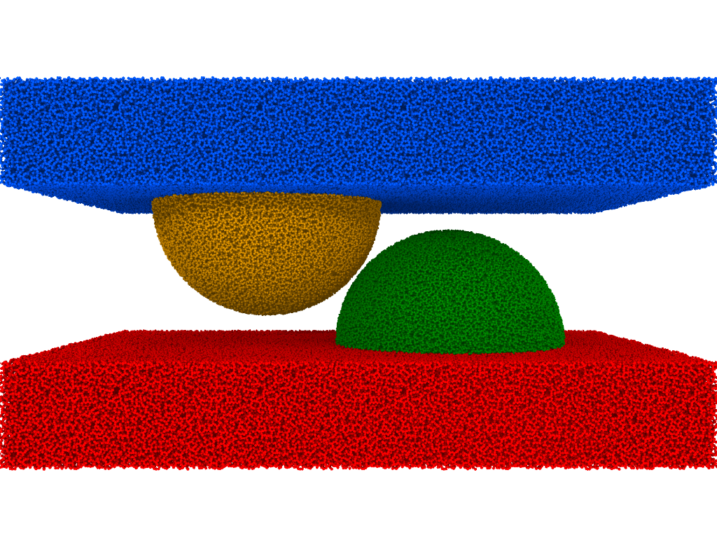
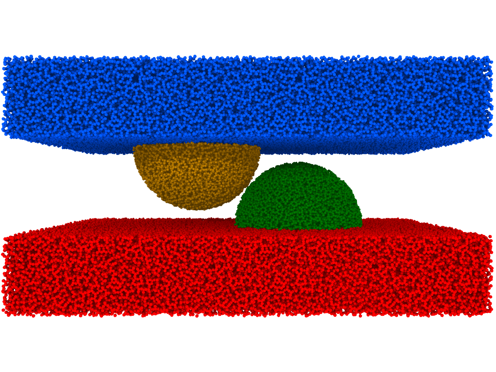
found for d∗is likely to also be quantitatively accurate. To confirm that the estimated d∗really corresponds to the transition of interest for amorphous SiO2, we simu- lated a setup equivalent to Aghababaei et al. using the Vashishta potential in LAMMPS.32 The setup consists of two hemispherical asperities of diameter d, each attached to a flat body (as shown in Figure 3(a)). The amorphous SiO2 structure is created following the same procedure as before. A periodic cubic unit cell of side ≈10 nm contain- ing amorphous SiO2 was generated and used to build the whole setup by tiling the space with the SiO2 cells and carving the desired shapes by removing the atoms, while making sure to preserve charge neutrality. A constant lateral velocity of 10 m/s is applied on the upper body to make the asperities collide. Normal loads are applied on the top and bottom bodies to obtain pressures of 100 MPa to 200 MPa on the loaded surfaces, which prevents the sys- tem from flying apart. Periodic boundary conditions are applied in the horizontal directions. Langevin thermostats are applied at the non-periodic boundaries to keep the temperature of the system constant at 300 K with a damp- ing constant of 0.01 ps. A timestep of 1 fs is used. The simulation results are shown in the Figures 3 to 5, visual- ized using OVITO,33 for the asperity diameters d = 7 nm,

D = 10 Nm And D = 20 Nm. These Values Were Chosen

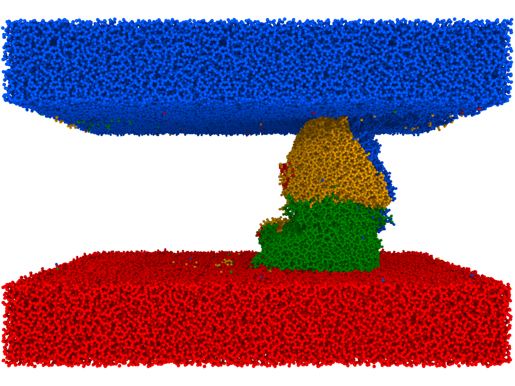
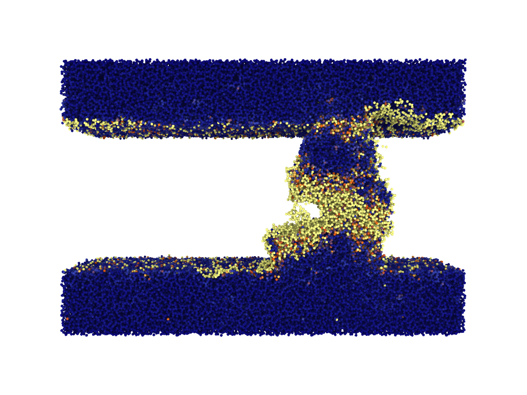
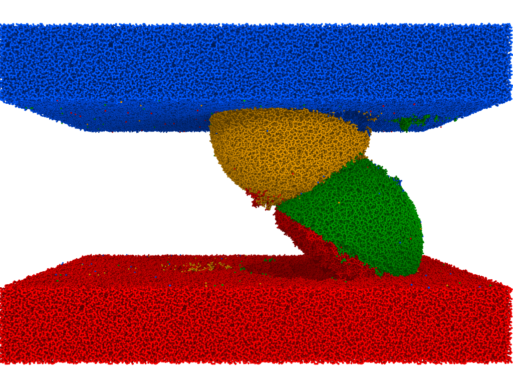
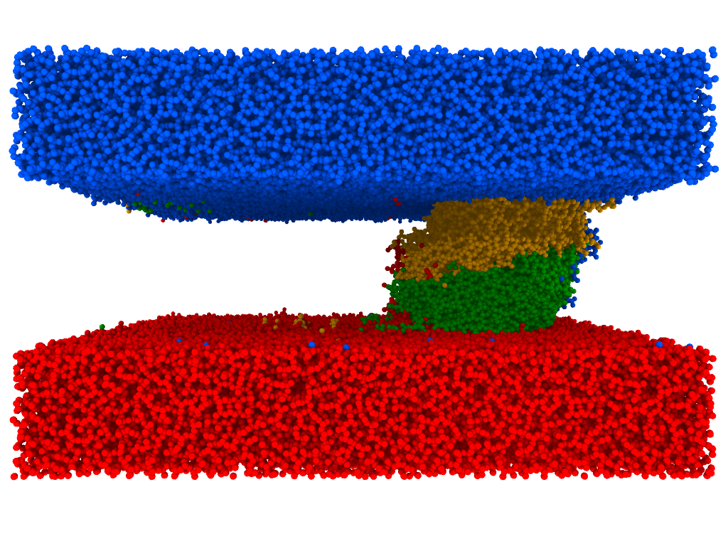
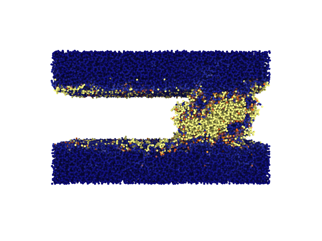
around the theoretical estimate d∗≈15 nm. The atomic shear strain (computed relative to the initial configura- tion) is used to determine whether the wear regime is ductile or brittle. In the ductile case (Figure 3), the collid- ing asperities are plastically deformed, resulting after the collision in high permanent shear strains between all the atoms located in the plasticized region. In the brittle case (Figure 5), a wear particle combining the two asperities is formed, and high strains only remain in the fractured regions, whereas inside the wear particle, the strains in- crease during the collision and return to a low value after the formation of cracks, since the atoms retain their orig- inal configuration. According to Aghababaei et al., the critical length scale d∗is defined as the size of the junction between the colliding asperities corresponding to the tran- sition between ductile and brittle behaviors. In our case, instead of measuring the size of the junction, we assume for simplicity that it has a size roughly equal to the diam- eter of the asperities d. The simulations show that the d∗ of amorphous SiO2 is indeed located between 7 nm and 20 nm. Note that there is no sharp transition between the ductile and brittle behavior (see Figure 4 which shows an in-between behavior), which is why d∗is called a length scale rather than a definite length.

The theoretical estimate d∗≈15 nm and the lower and

Upper Bounds (D∗> 7 Nm And D∗< 20 Nm) Found Using

simulations for the value of d∗for SiO2 are in line with the minimum size of wear particles found experimentally (no particles smaller than 30 nm were observed). This sup- ports the idea that no wear particles smaller than d∗can be created, which is expected because a junction smaller than d∗cannot be detached into a wear particle. Due to the na- ture of d∗being mainly dependent on material parameters and only weakly on geometry or loading conditions, we can infer that the minimum size of wear particles formed when rubbing two surfaces together is equal to d∗and similarly only dependent on the materials of the two sur- faces.

Having established the notion of minimum wear parti- cle size, we know that wear particles can be formed when two asperities located on rubbed surfaces and having a diameter greater than d∗collide into each other. There- fore, wear particles can understandably form from rough surfaces. The formation of wear particles is still possible if the surfaces are flat and free of protruding asperities.

When put in contact under a normal load, the surfaces will meet at some points and create adhesive junctions. A tangential load applied on an adhesive junction will enable the formation of wear particles if the size of the junction is greater than d∗. If it is smaller, the junction may grow in size due to plastic deformations, if the adhesive forces are strong enough, until reaching the critical size when a wear particle can finally be detached.

3.2. Roughness Formation

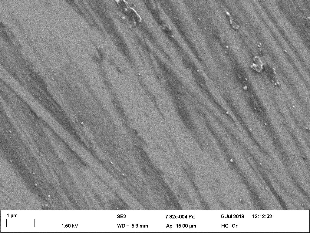
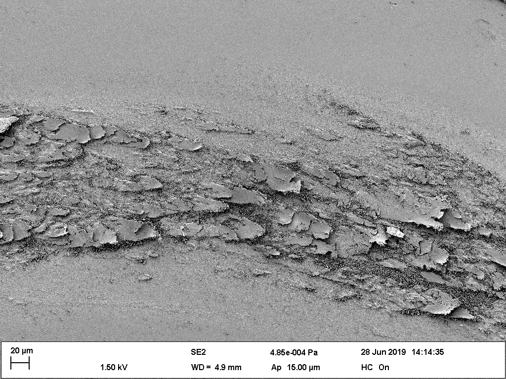
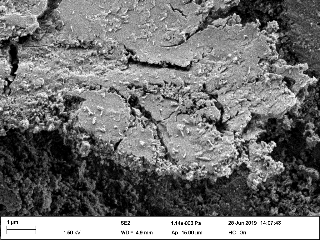
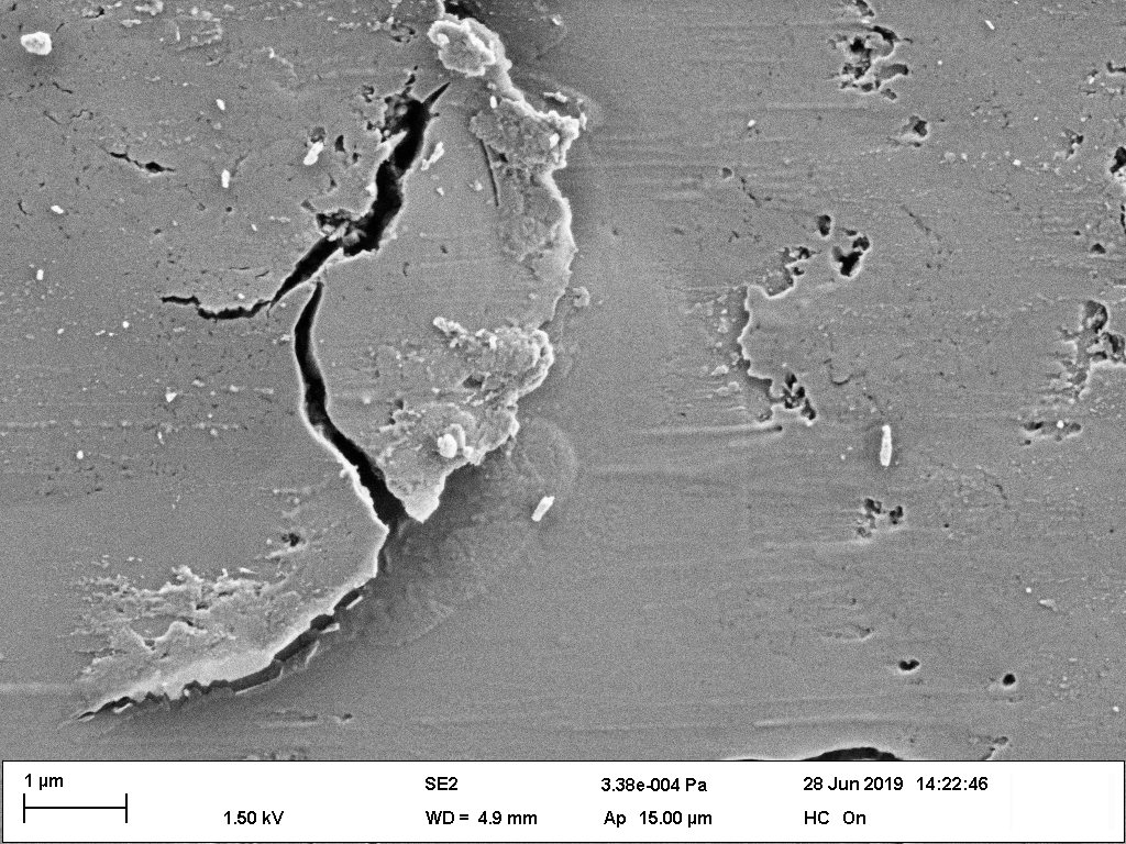
Figure 6 shows SEM images of the wear track left by a ball on flat discs after various sliding durations in chrono- logical order. From an initially almost flat surface of the disc, the process of creation of surface roughness goes through different steps. At first, small spherical wear par- ticles of minimum size d∗are created in the way described in the previous section (see Figure 2 and 6(a)). The newly created particles enter a rolling motion between the two rubbed surfaces and start growing in size by chipping away some material from the flat surfaces thanks to adhe- sive forces (larger particles in Figure 2). The increase of the diameter of the rolling spherical particles is limited by the normal pressure applied by the opposed surfaces, so that the spherical particles will instead continue to grow by elongating into rolling cylinders. With the current load- ing conditions, the cylinders reach a maximum length of about 500 nm and a maximum diameter of 100 nm (see Fig- ure 6(b)). When the cylinders become numerous and meet each other, they agglomerate into larger aggregates. The accumulation of aggregates takes the form of large flakes being left on the initially flat disc, creating a third-body or gouge layer and resulting in the macroscopic surface roughness. The flakes have an average width of 20 µm (see Figure 6(c)). The same mechanisms of wear forma- tion continue to take place on top of the already formed third-body layer, as seen in Figures 6(d) and 6(e), where

(C) Shear Strain (Cross Section)

Figure 3: MD simulation of a collision between two amorphous SiO2 asperities of diameter d = 7 nm. The initial simulation size is 20.2 nm × 21.0 nm × 11.8 nm (in the figures: length × height × depth). The non-localized shear strain (brighter is higher) shows a plastic deformation of the asperities, indicating that d < d∗.

(C) Shear Strain (Cross Section)

Figure 4: MD simulation of a collision between two amorphous SiO2 asperities of diameter d = 10 nm. The initial simulation size is 30.3 nm × 21.0 nm × 16.0 nm. The behavior is in-between ductile and brittle, indicating that d ≃d∗.

(C) Shear Strain (Cross Section)

Figure 5: MD simulation of a collision between two amorphous SiO2 asperities of diameter d = 20 nm. The initial simulation size is 50.5 nm × 31.6 nm × 27.5 nm. The presence of clear cracks (regions of high strain) indicates a brittle behavior, implying that d > d∗.

Outside The Wear Track

Figure 6: SEM images of wear tracks on flat discs after different amounts of time cylinders are visible on top of the large aggregated flakes. While the creation of wear particles and their accumu- lation into a third-body layer is commonly seen in engi- neering16,34–36 or at geological scales,37 the formation of rolling cylinders is interesting in itself and subject to re- cent discussions in litterature. Rolling cylinders have been observed in lubricated38 and unlubricated39,40 wear. In the latter case, the cylinders are believed to decrease the in- terfacial tangential stresses. Reches et al.41 have conducted rock friction experiments and observed the formation of rolling cylinders along the sliding direction. They believe the occurrence of these wear cylindrical bodies is a mech- anism that leads to slip weakening, with implications in earthquake physics.

3.3. Roughness Evolution

Figure 7 shows topographic images of disc surfaces with different initial roughnesses (one in each category of Table 1) acquired using a Sensofar S-Neox confocal micro- scope, before and after an experiment with a sliding dura- tion of 5 h. Initially, the roughened samples exhibit strong rough features, also revealing the direction of polishing.

After the experiments, a wear track is left on each disc, which is visible in the topographic images as well as to the naked eye. When the disc is initially flat, the resulting wear track is comparatively rougher (Figure 7(c)). Con- versely, when the disc is initially very rough, the rough- ness inside the wear track is decreased by the flattening of the high features (Figure 7(e)). In-between, when starting from a relatively moderate surface roughness, the created wear track keeps the same roughness, resulting in a topo- graphic image with uniform heights (Figure 7(d)).

This observed trend in the evolution of surface rough- ness can be complemented by more accurate topographic computations. Figure 8 shows measurements of friction coefficient and of the two-dimensional Sa roughness of the wear tracks left on the discs for all the tests listed in the Table 1.

The evolution of the friction coefficients indicates that an almost steady state is reached after a running-in pe- riod. The running-in period itself does not seem to last a constant time between the different tests. For example, the wear track on the disc can start to become visible to the naked eye on the initially flat discs after 30 seconds or only after 5 seconds of sliding for two repetitions of the same test. The running-in period may be very dependent on small non-controlled variations of the initial conditions (like dust, temperature or hygrometry). The friction coeffi- cient still increases slowly in the ‘steady’ region, which is probably linked to the non-constant contact area between the worn ball and the disc, which increases as the ball wears out.

The dashed curves of the Figure 8(a) are fitted to all the evolution curves of a given category of initial surface roughness of the disc (corresponding to the three cate- gories of the Table 1). Functions of the form a + bx + cedx are empirically chosen, only for visual comparison pur- poses, as they can represent a steadily increasing regime

Related Journal Articles & DOI Links

Selected peer-reviewed publications relevant to 12 Lead ECG Acquisition. Click the DOI to access the full paper (may require institutional access).

Why Choose Us?

Bangalore guidance for robotics, Spectre and autonomous systems projects.