Simulia Living Heart Electrophysiology

Electrophysiology Of The Whole Human Heart

Giulio Del Corsoa, Roberto Verziccoa,b,c, Francesco Violaa,∗ aGSSI (Gran Sasso Science Institute), L’Aquila, Italy

Abstract

In this study we present a novel computational model for unprecedented simu- lations of the whole cardiac electrophysiology. According to the heterogeneous electrophysiologic properties of the heart, the whole cardiac geometry is de- composed into a set of coupled conductive media having different topology and electrical conductivities: (i) a network of slender bundles comprising a fast conduction atrial network, the AV–node and the ventricular bundles; (ii) the Purkinje network; and (iii) the atrial and ventricular myocardium. The prop- agation of the action potential in these conductive media is governed by the bidomain/monodomain equations, which are discretized in space using an in– house finite volume method and coupled to three different cellular models, the Courtemanche model for the atrial myocytes, the Stewart model for the Purkinje Network and the ten Tusscher–Panfilov model for the ventricular myocytes. The developed numerical model correctly reproduces the cardiac elec- trophysiology of the whole human heart in healthy and pathologic conditions and it can be tailored to study and optimize resynchronization therapies or in- vasive surgical procedures. Importantly, the whole solver is GPU–accelerated using CUDA Fortran providing an unprecedented speedup, thus opening the way for systematic parametric studies and uncertainty quantification analyses.

Keywords:

electrophysiology, bidomain equations, heart modelling, GPU

Arxiv:2112.12854V1 [Physics.Med-Ph] 23 Dec 2021

computing.

1. Introduction

Owing to the development of accurate mathematical models capable of vir- tually replicating biological systems and to the growing availability of computa- tional resources to solve them, medical research is increasingly integrated with computational engineering . In particular, the correct modelling of the heart functioning in healthy and pathologic conditions – such in the case of ischemic events (reduced blood supply to a portion of the myocardium leading to dys- function and, possibly, to the necrosis of the tissue) or of bundle branch block (delay or blockage along the heart electrical pathway) – entails reproducing the highly cooperative and interconnected dynamics of the heart, including its com- plex electrical activation.

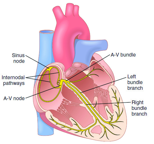
The latter involves many embedded conductive structures with different bi- ological properties so as to rapidly propagate the electrical activation of atria and ventricles in order to achieve an efficient muscular contraction propelling the blood into the circulatory system. As shown in Figure 1 a), the cardiac elec- trical depolarization, corresponding to a rise in the electrical potential across the cellular membrane owing to the transmembrane flux of ions, is initiated close to the entrance of the superior vena cava at the sinoatrial node (SA–node). Within the SA–node, some specialized pacemaker cells spontaneously produce a peri- odic electrical impulse, the action potential, which propagates across the right atrium through three high speed conductivity bundles – namely the Thorel’s pathway/posterior internodal tract, the Wenckebach’s middle internodal tract and the anterior internodal tract – that wrap the right atrial chamber to assure a uniform activation. A branch bifurcating from the latter bundle then penetrates into the internal muscle of the left atrium (Bachmann’s bundle), thus initiating the depolarization also of this chamber.

Since The Propagation Speed Of The

action potential within the fast internodal bundles is of about 1–2 m/s (signif- icantly larger than the one observed in the atrial muscle of about 0.3–0.5 m/s

2

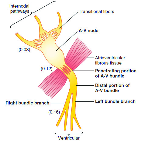
[5, 6, 7]), after 30 ms the depolarization front reaches the atrioventricular node (AV–node) which is the electrical gate connecting the atrial with the ventricular electrophysiology system, see Figure 1(b). In the AV–node, specialized cells slow down the propagation of the transmembrane potential by about 100 ms in order to allow both atria to contract before the activation wave reaches the ventricles; this avoids the simultaneous contraction of the whole organ which would pro- duce inefficient filling/emptying of the four chambers and impaired pumping .

Once beyond the AV–node, the signal propagates through the His bundle, which forks into the right and left bundle branch that, in turn, progressively divide into a plethora of thin, tightly woven specialized cells named the Purkinje network, where the propagation speed of the action potential is in the range 1.5-4 m/s, corresponding to six times the propagation speed in the ventricular muscle .

This fast conduction system quickly propagates the electrical signal within the ventricular myocardium (about 30 ms to reach the terminations of the Purkinje fibers) to provide an almost simultaneous contraction of the ventricular muscle.

In addition, the Purkinje network also assures the timely activation of the pap- illary muscles, which stretch the chordae tendineae so to prevent the eversion of the mitral and tricuspid valve leaflets by pulling down their free margins dur- ing early systole . Although the precise morphology and orientation of the Purkinje network can not be measured in–vivo, a significant variability among individuals is known to exist , also depending on the positions of the papillary muscles which also varies among the population . Furthermore, its smaller fibers are randomly oriented in the subendocardium with a penetration length in the myocardium of about 0.5 −100 µm and with an average distance among them of about 0.1 mm [12, 13]. The Purkinje fibers are electrically isolated from the myocardial muscle, except at their endpoints called PMJs (Purkinje Muscle Junctions), where the electrical signal can propagate from the Purkinje fibers to the ventricular myocardium with a delay ranging from to 5 to 15 ms (ortho- dromic propagation) and vice–versa from the myocardium to Purkinje with a delay of 2-3 ms (antidromic propagation) .

Both the fast bundles and the Purkinje networks electrically activate the

B)

Figure 1: Sketch of the electrophysiology system of the heart . a) Fast conduction networks of bundles and Purkinje. b) Detail of the AV bundle with the corresponding activation times (in seconds) showing the propagation delay happening in the AV–node.

muscular myocardium in terms of action potential, which then propagates in the thick muscular myocardium at a lower speed that depends on the local fiber orientation. The myocardium is, indeed, an orthotropic medium made of oriented myocytes that enable a faster transmission of electrical impulses in the fiber direction than in the orthogonal one and this tissue heterogeneity, playing a role in the atrial and ventricular [17, 18] depolarization, should be ac- counted for in cardiac numerical models. According to the model proposed by Buckberg et al. the muscular fibers have a dual-orientation, with directions ranging approximately from +60◦to −60◦across the ventricular wall and this structure has been confirmed by accurate imaging analysis of mammalians heart . An additional cause of inhomogeneity is that the ventricular my- ocytes have different electrical properties from the atrial ones, thus resulting in a different electrical conductivity (yielding a different propagation speed) and different ionic fluxes across the myocytes membrane, which entail a different contraction pattern of atrial and ventricular chambers.

In the last decades few mathematical models for solving the cardiac elec- trophysiology have been proposed.

The Eikonal Approach Solves Directly The

electrical depolarization of the cardiac tissue by taking as input the propaga- tion speed within the media , whereas the interconnected cable methods

4

solve the propagation of an electrical stimulus thorough a connected network of discrete cables representing the myocardium [23, 24]. These methodologies have a limited computational cost and have been used to model the cardiac tissue including the macroscopic effects of structural heterogeneity on impulse propagation and to incorporate more complex conduction structures, such as cardiomyocytic fibers orientation and the His–Purkinje activation network . On the other hand, leveraging on the continuum hypothesis the cardiac tissue can be modeled as an intracellular and an extracellular overlapping con- ductive media separated by the cell membrane. The resulting bidomain model [27, 28] thus consists of the coupling between a system of reaction–diffusion partial differential equations (PDEs, governing the potential propagation in the media) and a set of ordinary differential equations (ODEs) for the cellular ionic model describing the current flow through ion channels. The bidomain model is the state–of–the–art mathematical model for reproducing the cardiac electro- physiology at a continuum level [29, 30], it has been validated against several experiments on animals [31, 32] and it is currently adopted to solve the action potential propagation in healthy and pathologic conditions including ischemic events and fibrillation [33, 34, 30]. In the case the extracellular conductivity tensor is proportional to the intracellular one, the bidomain equations can be simplified into a single governing equation for the transmembrane potential, the monodomain system, which is computationally cheaper than the bidomain counterpart as the number of degrees–of–freedom (dofs of the system of PDEs) is halved . Unless complex pacing patterns or fibrillation are present, the monodomain equation can be conveniently used to approximate the bidomain solution also in the case the conductivity tensors are not proportional by setting the components of the monodomain conductivity tensor to half the har- monic mean of the corresponding extracellular and intracellular components .

The bidomain/monodomain electrophysiology model has been widely used to study different components of the cardiac electrical network such as the atrial depolarization also including pathologic atrial fibrillation [36, 16] or to model

5

the AV–node depolarization [37, 38]. The depolarization in the ventricular my- ocardium has been investigated in a series of works [17, 39, 40, 41] also including the fast conduction Purkinje network [14, 21, 42], which is needed to reproduce a realistic ventricular depolarization, especially in the presence of infarction or reentry initiation of arrhythmias [44, 45, 46]. In these works, the geometry of the Purkinje network is generally obtained by applying a growing algorithm to a one–dimensional (1D) network of fibers, which has to be sufficiently dense in order to correctly activate the 3D myocardium [47, 48, 49].

Although some studies are very advanced in solving the bidomain/mon- odomain equations in a portion of the cardiac electrical network [50, 51, 52, 53, 54], a comprehensive computational framework, solving simultaneously the fast conduction electrophysiology networks and the four–chambers muscular my- ocardium, is still missing. Such a computational model for the whole cardiac electrophysiology would entail, indeed, the solution of a large dynamical system, thus calling for efficient code parallelization with an effective use of the com- putational resources. This work aims at building an accurate computational framework for solving the whole cardiac electrophysiology accounting for: (i) the fast conductivity structures of the atria and ventricles including the intern- odal pathways, branch bifurcations, and the AV–node; (ii) the Purkinje network immersed in the ventricular myocardium, which activates the ventricular mus- cle at the PMJs; (iii) the thick atrial and ventricular myocardium with their muscular fibers orientation yielding electrical anisotropy. These three electrical components of the system have different electrophysiology properties and are modelled using a hierarchy of interconnected geometries having different topo- logical dimension and cellular models. The bidomain/monodomain equations are discretized in space using an in–house finite volume method that allows for tackling complex geometries, also deforming in time, and the whole model has been ported to CUDA to run on GPU architectures thus providing unprece- dented speedups [55, 4]. The resulting computational model is then applied to solve the cardiac electrophysiology in healthy and pathologic conditions with the aim of assessing the model performance and validating its results.

6

The paper is organized as follows.

After The Introduction Of The Cardiac

geometry used throughout the work in § 2, the governing equations and the GPU–accelerated numerical methods are detailed in § 3. The convergence anal- ysis of the code and validations against benchmarks results from the literature are reported in § 4. In § 5 the electrophysiology activation of the whole human heart is studied in healthy and pathological conditions, including bundle branch blocks and the implant of artificial cardiac pacemakers. Conclusions and fur- ther research directions including possible uncertainty quantification analyses are outlined in § 6.

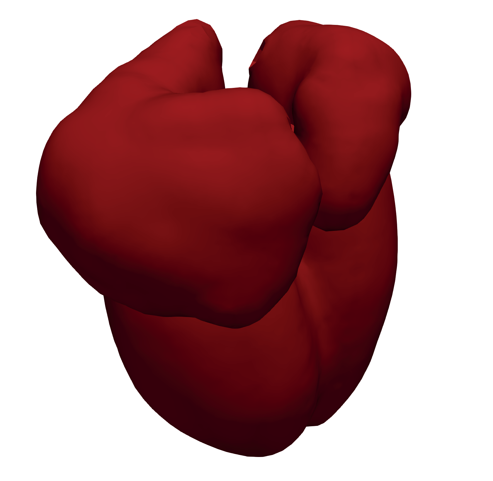
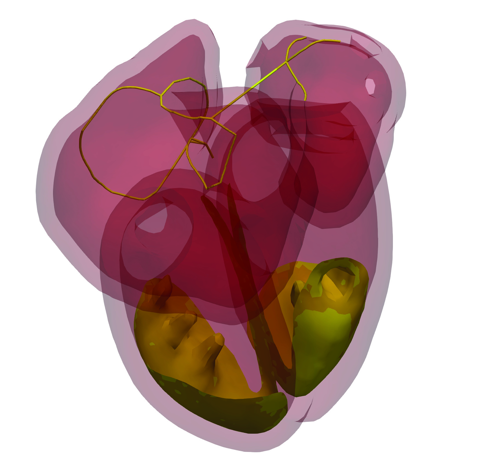
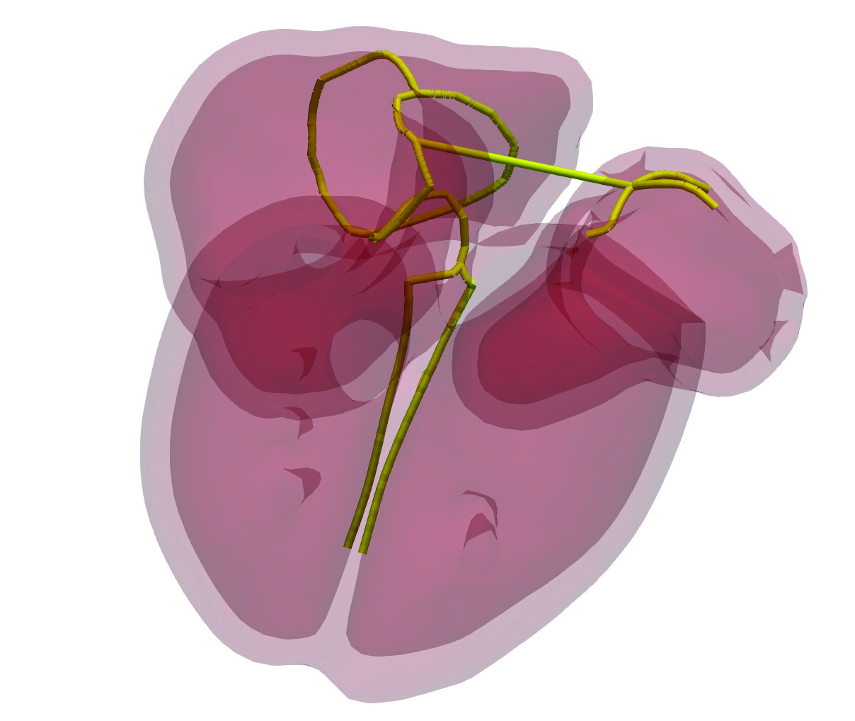
2. Computational domain: splitting the electrophysiology system Figure 2: The a) whole cardiac electrophysiology system is split in: b) 1D network of fast conduction bundles, c) 2D Purkinje network and d) 3D myocardium.

As anticipated above, the cardiac electrophysiology system is made of a (i) fast conduction network of bundles, (ii) a Purkinje network for the ventricular

7

activation and (iii) the massive conductive myocardium contracting as the my- ocytes depolarize. Our computational approach is based on intrinsic connections among different conductive media and pathways, and the complex electrophys- iology system is thus split in several interconnected subdomains with different dimensional topology (see Figure 2), namely a one–dimensional graph (1D) mod- elling the fast conduction bundles (panel 2 b); a two–dimensional (2D) surface approximating the dense Purkinje network (panel 2 c); three-dimensional (3D) media for the atrial and ventricular muscles (panel 2 d). The solution of the complete system, shown in panel 2a, is thus obtained by the coupled solutions of these three distinct components which are detailed in the following.

2.1. One dimensional fast conduction network of bundles

Figure 3:

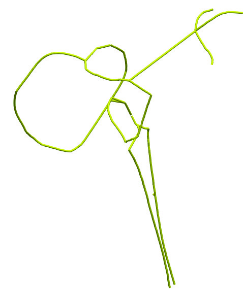
Fast conduction network of bundles. The circles indicate the geometrical control points of the atrial network (blue), AV–node (green) and ventricular network (red). Owing to its slenderness, the fast conductivity structures conveying the elec- trical signal through the 3D myocardium has been modelled as a 1D fast con- duction pathway with space–varying electrophysiology properties (see Figure 3).

The network originates from the SA–node and branches into the three internodal pathways reaching the AV–node with one of them (the anterior internodal path- way) further branching and connecting the right atrium to the left one through

8

the Bachmann’s bundle. The terminations of the internodal pathways reach the AV–node (in two locations) connecting the atrial fast conduction network with the ventricular through the bundle of His, which then splits into two distinct branches, one immersed in the right ventricle and the other in the left one.

In order to eventually adapt the fast conduction network to different pa- tient geometries, the entire graph is generated through a set of control points whose coordinates can be arbitrarily set so to easily reproduce a given cardiac geometry following the adaptive procedure. Specifically, 19 control points are distributed among the SA–node and the atrial bundles (indicated by blue bullets in Figure 3), 4 control points are used for the AV–node and its connection with the bundle of His (green bullets in Figure 3) and 7 more control points are used for the ventricular bundles (red bullets Figure 3). The pathways connecting the control points are built using a piecewise linear interpolation which are then projected over the atrial and ventricular endocardium, whereas the portions of the 1D graph lying within the ventricular septum, such as the AV–node, are im- mersed in the 3D mesh volume. The 1D graph is then meshed uniformly with linear elements of a given grid size (much finer than the distance between two adjacent bullets). The whole procedure runs in few CPU–minutes, thus provid- ing the correct positioning of a realistic 1D conduction network within the 3D mesh, with multiples bundles branching/joining the same nodes, as shown in Figure 3.

2.2. Two Dimensional Fast Conduction Purkinje

The Purkinje network in humans and other mammals is distributed in a layer within the subendocardium, which is thin with respect to the myocardium thickness (of the order of 0.5–100 µm compared to an average thickness of 7±1 and 15.4±2.3 mm for the right and left ventricles, respectively ) and is made of thicker fibers with a branching distance of the order of 2 mm which bifurcate multiple times until forming a dense plethora of thinner fibers [47, 59].

This dense network of fibers is typically mimicked in computational models through the growth of a fractal structure by defining a set of generating rules

9

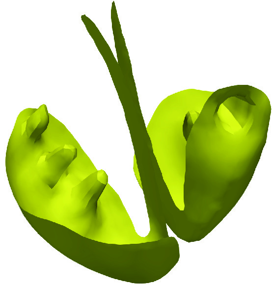
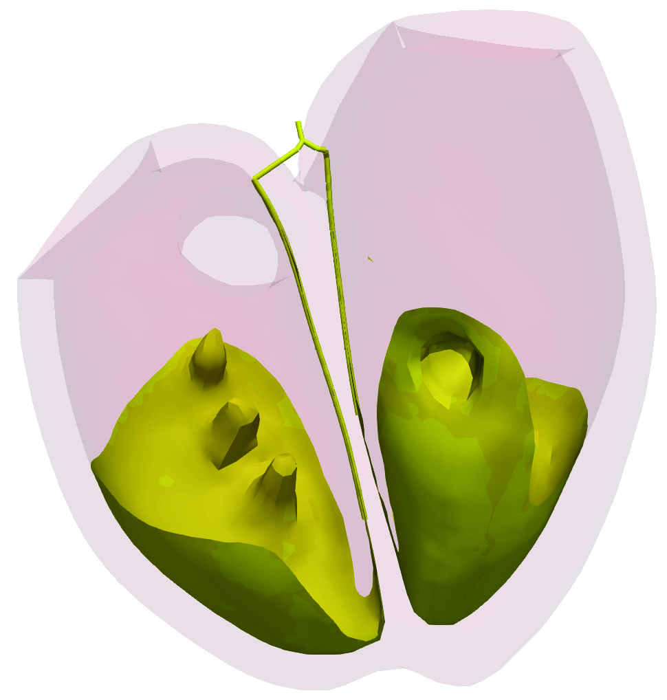
Figure 4: Ventricular bundles and Purkinje network, which cover the papillary muscles. and an initial topology (in a similar fashion to the growing models for plant branches) with the smallest branching structure in the order of 100 µm [47, 12, 13]. As an alternative approach to the growth of a fractal 1D network, the dense fiber distribution of the Purkinje network is here merged into a continuum 2D isotropic conductive medium wrapping the endocardium. Such approach is motivated by the uncertainty on the precise arrangement of Purkinje fibers and the great variability among individuals, which make it difficult to develop an accurate fractal rule for the network growth. Furthermore, a high fiber density (more than 2000 branches and 300 PMJs for the major bundles and an even smaller branching distance of 0.1–2 mm for thinner branches [58, 47]) is required to adequately model the Purkinje and correctly activate the myocardium both in healthy and pathologic cases. Figure (4) shows as the 2D Purkinje network develops from the His bundle and extends parallel to the left and right bundles until reaching the apex of the heart and then raises up upon two third of the ventricles height, completely covering the papillary muscles in order to timely activate their contraction at early systole. The right and left sides of the Purkinje complex do not have a direct electrical connection since they are separated by the thickness of the interventricular septum.

2.3. Three Dimensional Excitable Myocardium

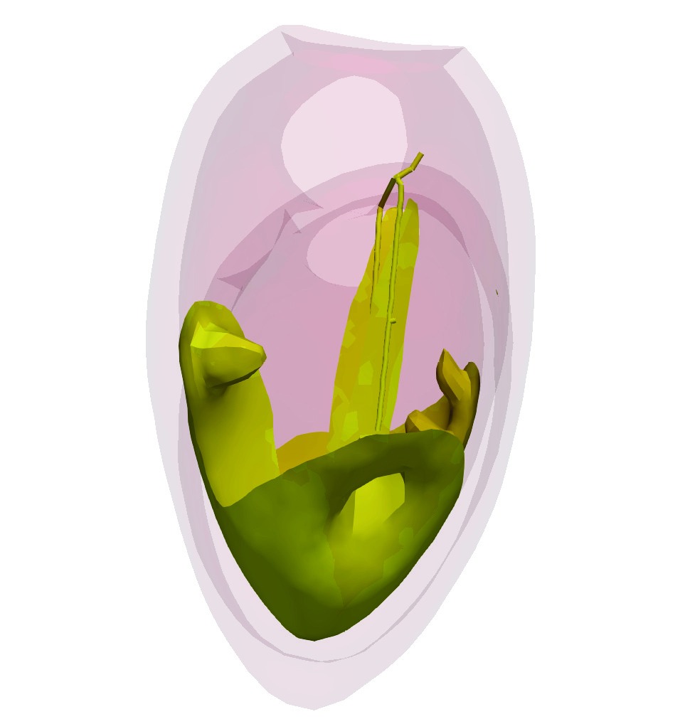
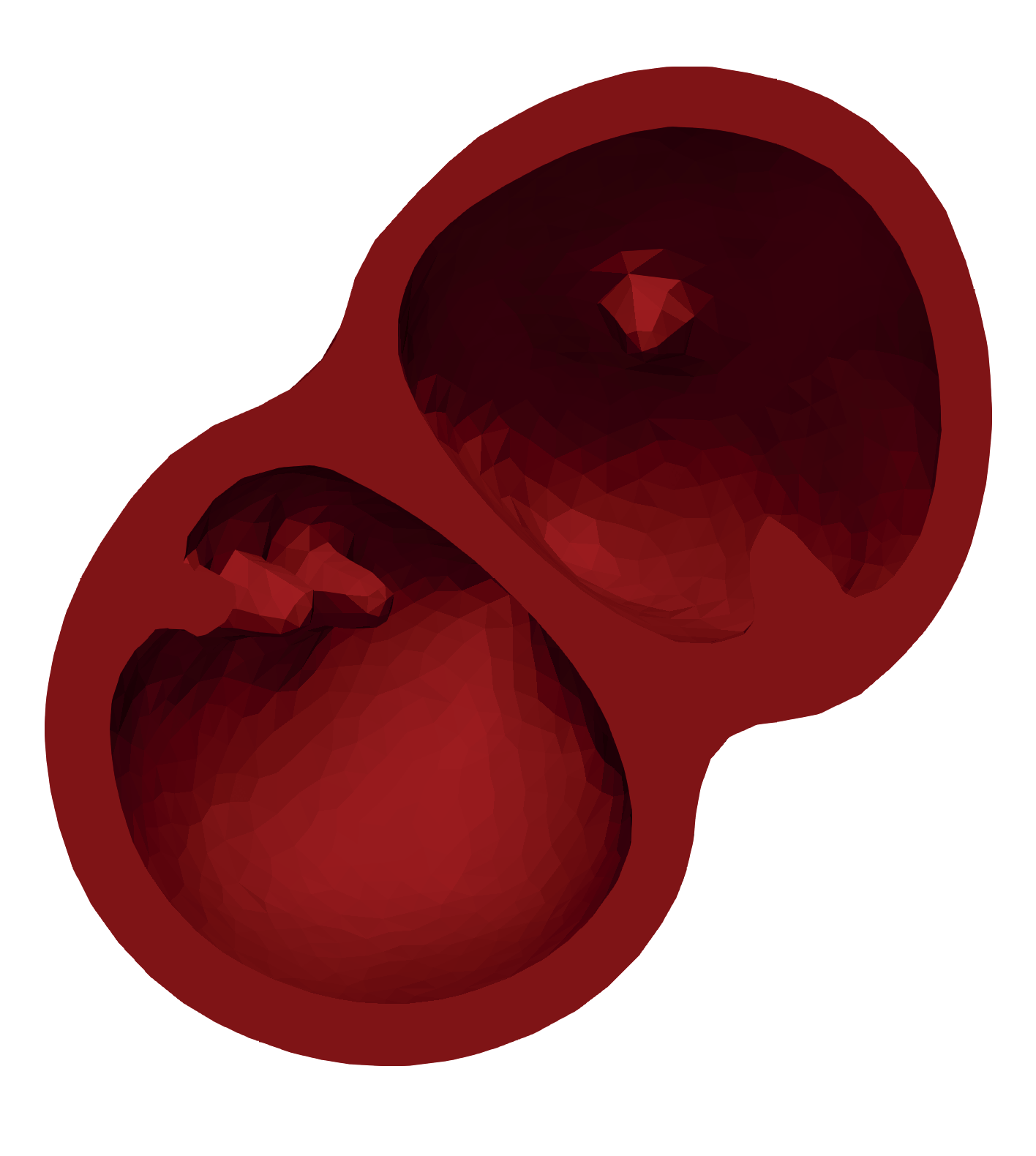
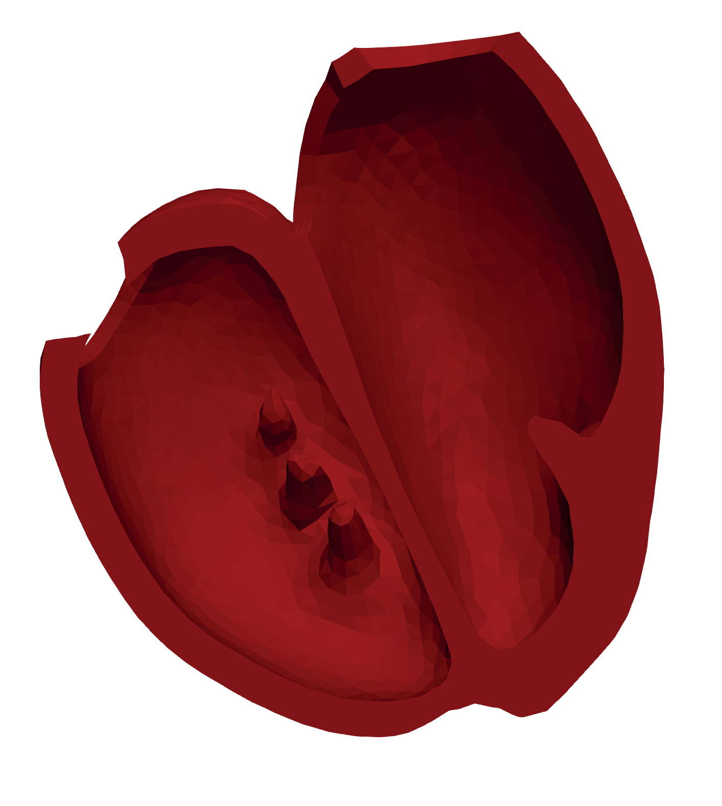
The 3D myocardium is made of three excitable and conductive media, namely two for the left and right atria and another for the ventricles (see Figure 2d), which has been built using modeling software so as to reproduce high–resolution clinical images and medical atlas. This splitting of the myocardium is inspired by the cardiac electrophysiology as the heart septum between the atria and the ventricles (the fibrous trine plane) acts as an electrical insulator, thus decoupling the atrial and the ventricular electrophysiology. The transmembrane depolar- ization front, indeed, only propagates from the atria to the ventricles through the AV–node that is part of the 1D network of bundles (see § 2.1). Similarly, the atria are electrically insulated by the atrial septum and they can thus be modelled as two disjoint electrical domains. On the other hand, the ventricular myocardium cannot be further subdivided into two independent meshes as, we anticipate, the ventricular endocardium is made by the same muscular fibers wrapped around the ventricles which are thus electrically connected .

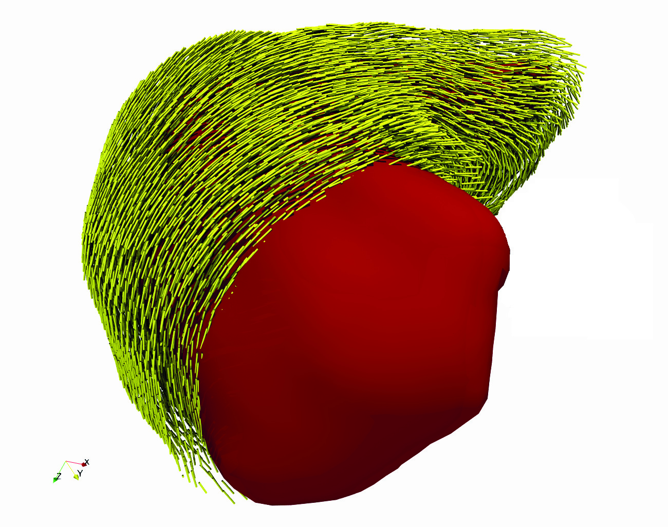
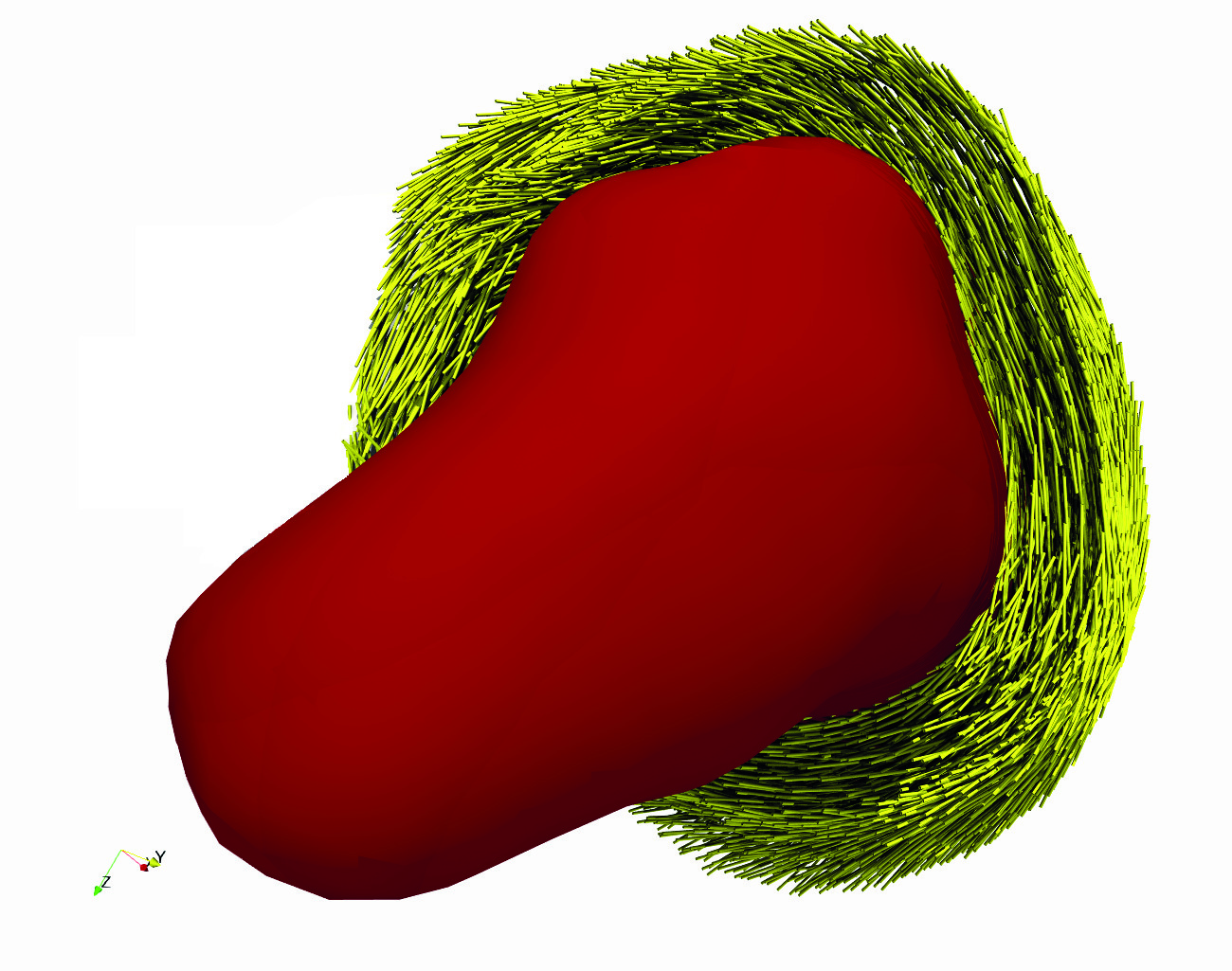
Figure 5: Fibers orientation in the a) right and b) left atrium. The red surface indicate the internal endocardium. Figure 5 shows the muscular fibers orientation within the (a) right and (b) left atrial wall, with the fibers wrapping around the main atrial axes as observed in–vivo by diffusion tensor magnetic resonance . Since the atrial fiber orien- tation is uniform within the myocardium thickness (of about 4 mm), this is first

11

defined on the atrial endocardium (red surfaces in Figure 5) and, then replicated, at each cell across the 3D myocardium thickness. Different or patient–specific fiber orientation in healthy and pathological conditions can be included as well in the geometrical description of the 3D media.

Figure 6: a) Front and b) top view of the ventricular myocardium incorporating the papillary muscles. The ventricular myocardium is modelled as a single 3D mesh for both the left and right ventricles and includes the papillary muscles, whose location cor- responds to the most recurrent one observed in a population study [61, 62].

The main reason for creating a single mesh (instead of two as in the modelling of the atria) is that the external part of the ventricular myocardium wrapping the whole heart (often described as a scarf ) is electrically connected and allows for a slow propagation of the depolarization front from one ventricle to the other, which is not observed in healthy cases as the two ventricles are simul- taneously activated by the right and left fast conduction branches but it may occur in pathologic cases as studied in the next section.

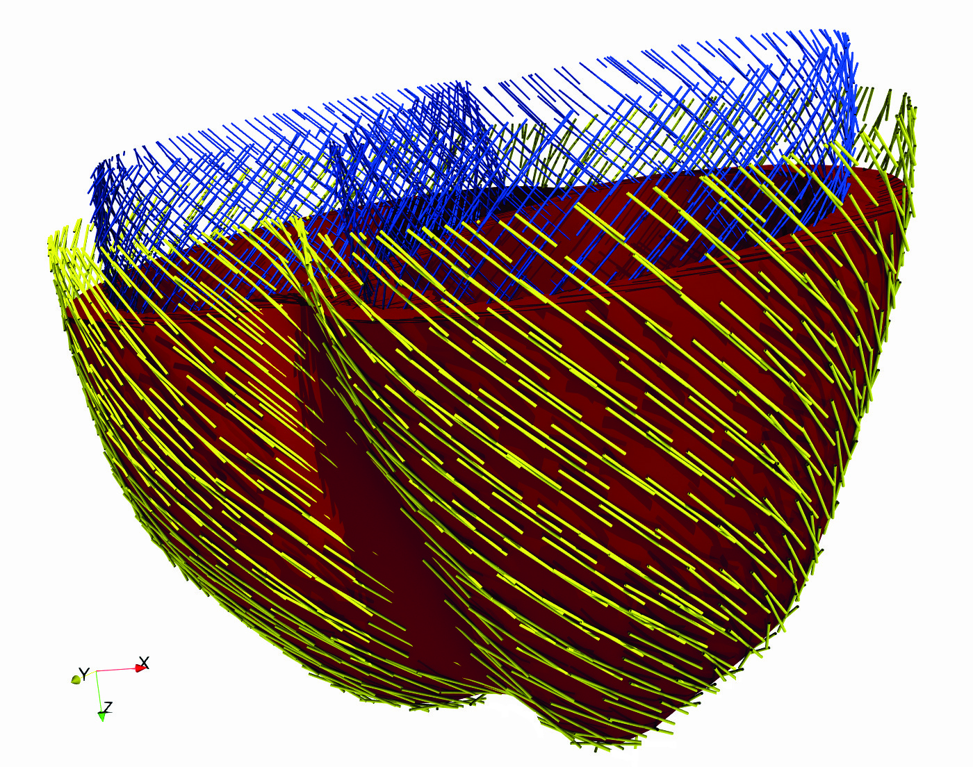
Although the orientation of the muscle fibers shows some variability among individuals, it is known to vary across the myocardium wall from αepi = 60◦at the endocardium to αendo = −60◦at the epicardium with respect to the ventri- cles major axis [20, 63, 64]. The vector field, corresponding to the fibers orien- tation at each cell of the 3D mesh, is thus defined as α = αendo ·d+αepi ·(1−d),

12

Figure 7: Fibers orientation in the ventricular myocardium. The external (yellow) epicardial muscular fibers are oriented in opposite direction compared with the internal endocardial one (blue).

where d is the cell transmural distance from the endocardium normalized by the myocadium thickness (of about 8 mm on average), yielding the typical counter- clockwise (clockwise) fiber orientation over the epicardium (endocadium) shown in Figure 7.

3.1. The Bidomain Model

The electric wave propagating across the cardiac tissue is governed by the bidomain model that is made by the following system of two reaction–diffusion PDEs, coupled with a set of nonlinear ODEs corresponding to the cell model:

∂S

∂t = F(v, s).

(1)

Here, v and vext are the unknown transmembrane and extracellular potential (expressed in mV ), whereas the surface–to–volume ratio of cells χ = 140 mm−1 and the specific membrane capacitance Cm = 0.01µF mm−2 are set as in .

13

M int and M ext are the conductivity tensors of the intracellular and extracellu- lar media that depend on the local fiber orientation with a faster propagation velocity along the fiber than in the orthogonal directions. In the case of a 3D conductive media as the myocardium these tensors have rank three and are diagonal when expressed in the fiber (∥), sheet–fiber (/) and cross–fiber (⊥)



.

(2)

The conductivity tensor in the global coordinate system are thus obtained by

(3)

where A is the rotation matrix containing column–wise the components of fiber, sheet–fiber and cross–fiber normal unit vectors. On the other hand, for 2D elec- trical media as the Purkinje model, the transmembrane potential depolarization can only propagate in the fiber and sheet–fiber directions corresponding to the

. Lastly, In The Case Of 1D Conduc-

tive media as the fast conduction network of bundles, the conduction properties

∥

. The last of equations (1) indicates the cellular model depending on the state vector s, which couples the cellular model with the bidomain equations through the ionic current per unit cell membrane Iion (measured in mA/mm2). Since the various components of the cardiac electrophysiology system have different cellular properties yielding different ionic fluxes and, consequently, different ac- tion potential profile, we adopt a Courtemanche cellular model for the atrial myocytes (and the corresponding internodal pathways), a Stewart model for the Purkinje network and a ten Tusscher–Panfilov model for the ventricular myocytes. The ionic current, Is gives to a periodic electrical stimulus concen- trated in time and space at the SA–node triggering the electrical stimulus to the

14

ventricular myocardium, thus initiating the electrical depolarization throughout

(4)

where Sa = 1 mA/mm2 and Sd = 2.5 ms are the stimulus amplitude and duration, t is the time within a heart beat and H[·] the Heaviside function. In a previous work, we have verified through an uncertainty quantification analysis that the values of the amplitude and duration of the stimulus do not significantly impact the subsequent depolarization of the fast conducting bundles, as far as they vary in physiological ranges .

3.2. Numerical Method

The set of governing equations (1) is solved using an in–house finite volume (FV) library, which provides a suitable approach for solving the electrophysiol- ogy equation in complex geometries. As introduced above, the cardiac electro- physiology media is split in a 1D graph for the fast conduction bundles, a 2D shell for the fast conduction Purkinje and 3D media for the atrial and ventric- ular myocardium, which are respectively segmented with linear, triangular and tetrahedral elements.

Using the divergence theorem, the bidomain equations (1) can be rewritten

(5)

where n is the normal unit vector of the cell boundary, ∂Ωi. In the case of the 3D myocardium, the domain is discretized through a tetrahedral mesh and equation (5) for a cell based FV method reads

E)

Figure 8: Graphical scheme of the procedure to evaluate the gradient at the cell faces of a 3D media. a) The cell—based vc is interpolated to obtain b) the node–based vn, which is then used to estimate the same quantity at c) the midpoint of the tetrahedrons faces, vf. The latter is used to determine d) ∇vc on the cell center using the Gauss–Green theorem and is successively interpolated to evaluate the e) gradient at the mesh faces ∇vf.

where the subscript c indicates that the quantities are evaluated at the cell center whereas the subscript fj denotes the j−th face of the cell c, see . In the case the external and the internal conductivity tensors are parallel M ext = λM int the bidomain model (6) reduces to the monodomain equation (6):

(7)

where M = λM int/(1 + λ). The fluxes over the tetrahedron cell faces are evaluated as indicated in Figure 8.

Firstly, the transmembrane potential at the vertex nodes vn (see panel 8 b) is computed by using the weighted average of the potential within the cells surrounding that node, vk, yielding vn = PNcn

K , Where

Ncn is the number of cells sharing the node and dk is the distance between the node and the k–th cell center. Once the values vn are found, the values of the transmembrane potential at the faces centroids vf (see panel 8 c) are calculated by averaging the three nodal values at the triangle vertices. Accord- ing the Gauss–Green formula (panel 8 d), the gradient of the transmembrane potential ∇vc is related to the flux of the same quantity through the cell faces and assuming that the transmembrane potential is uniform over each mesh

P4

j=1 vfjSfjnfj, where Vc is the volume of the cell and vfj, Sfj, nfj, are the transmembrane potential, area and the normal vector at j–th face. The gradient at the mesh faces is then obtained as the weighted

16

average of the cell gradients defined at the cells c1 and c2 sharing the face f, ∇vf = αc1∇vc1 +αc2∇vc2 where αc1 and αc2 are the linear interpolation weights defined on the position of the face f with respect to the centers of the two cells (αc1 +αc2 = 1). The resulting face gradient ∇vf is computed not only using the two transmembrane potential values defined at the two cells sharing the face, but also using the cell values of all the cells sharing the nodes of the two cells c1 and c2, thus enlarging the stencil of the formula. The 3D face gradient ∇vf, can be modified in such a way to include the low–stencil directional derivative and improve the stability of the method as follows

(8)

corresponding to the last panel in Figure 8. The face gradient (8) can be then directly used to compute the fluxes in the conservative equation (1) and obtain the spatially discretized bidomain equations in the 3D myocardium. A similar FV approach is used to discretize the bidomain/monodomain equations over 1D and 2D media (in order to model the bundles and Purkinje network, respec- tively) with the only exception that a vertex–based FV is used in the 1D case so to better handling multiple bundles branching from the same grid node, as happening at the internodal pathway and at the Bachmann’s bundle (see Fig- ure 3).

This FV approach thus provides an effective spatial discretization of the bidomain equations over complex geometries and is second–order accurate in space provided the grid is sufficiently regular (see the convergence analysis in section 4). Importantly, as typical in FV methods the mass matrix is diagonal, thus meaning that in the case of an explicit time scheme, the discretized un- steady bidomain equation for v (as well as the monodomain one) can be marched in time simply correcting the transmembrane potential at the previous timestep by summing an incremental vector. Although an explicit temporal scheme needs a timestep small enough to prevent numerical instabilities, still the overall com- putational cost is smaller than that of an implicit scheme which requires the solution of a nonlinear system at each mesh element and any timestep owing

17

to the nonlinearity of the cellular model. However, the cellular models are ex- tremely stiff, due to the significant variables variations over short timescales of the spike–and–dome of the action potential and of the so–called gating variables (describing the opening and closing dynamics of ion channels) and require pro- hibitively small timesteps to assure numerical stability. This difficulty can be circumvented by noting that the ODEs governing the gating variables are quasi- linear and can be solved analytically within a timestep if the transmembrane potential v is held constant, whereas an explicit method is used to integrate the remaining nonlinear ones. This semi–analytical approach is known as the Rush–Larsen scheme [68, 69] and it has been successfully applied to the three cellular models adopted here: the Courtemanche model with 15 gating variables out of 21 state variables, the Stewart model with 13 gating variables out of 20 state variables and the ten Tusscher–Panfilov models with 13 gating variables out of 19 state variables. The enhanced stability properties of the method thus allow for an integration timestep more than one order of magnitude larger than the one used with a standard explicit time scheme.

On the other hand, owing to the first order accuracy of the Rush–Larsen so- lution, the non–gating variables of the cell model (typically describing the varia- tions of intracellular ions concentrations) and the spatially discretized bidomain equations (6) are integrated in time using a forward Euler method and at each timestep the updated transmembrane potential v(tn+1) is thus obtained as an explicit function of v, vext, Iion and Is previously computed at time tn and, similarly, the updated state vector of the cellular model sn+1 is computed using sn. As the numerical converge analysis (see section 4) reveals that the error of the numerical solution is more sensitive to the spatial rather than to the temporal refinement, the Rush–Larsen method with its remarkable stability properties is thus a convenient temporal scheme for the bidomain/monodomain model, although first order accurate. Furthermore, in the perspective of multi- physics heart simulations including the coupled structural and blood dynamics, the timestep will be limited to few µs by the fluid–structure–interaction and a first order temporal scheme for the electrophysiology system entails a

18

numerical precision of the solution with such a small timestep.

In The Case

of bidomain model, once v(tn+1) is solved, the external potential vext(tn+1) , is obtained by solving the linear system given by the second equation of the system (6) through an iterative GMRES method with restart using the ex- ternal potential computed at previous time, vext(tn), as first estimate for the unknown field vext(tn+1).

The FV library has been GPU accelerated using CUDA Fortran which extends Fortran by allowing the programmer to define Fortran functions, called kernels, which when called are executed N times in parallel by N different CUDA threads, as opposed to the serial nature of the regular Fortran functions, thus greatly improving the performance. Furthermore, CUDA provides CUF kernel directories which automatically run single and nested loops on the GPU device without neither modifying the original CPU code nor writing a dedicated GPU subroutine. Specifically, the electrophysiology solver results in a sequence of loops on the mesh cells and on the mesh faces, which are GPU accelerated simply wrapping the original CPU code in the CUF kernel directive.

Front

Figure 9: Sketch of electrical coupling between the 1D fast conduction bundles and the sur- rounding 2D (or 3D) mesh. The wave front of the electric potential propagates across 1D mesh causing the threshold values of the communication nodes to be exceeded, thus activating the 2D (or 3D) cells within a radius Rs.

19

The topological splitting of the cardiac electrophysiology network requires a coupling mechanisms to connect electrically the various subdomains. In partic- ular, three two–way couplings are needed: (i) a first one between the 1D bundles and the 2D Purkinje networks, (ii) another between the 1D network of bundles and the 3D atrial myocardium and (iii) a last one between the 2D Purkinje and the 3D ventricular myocardium.

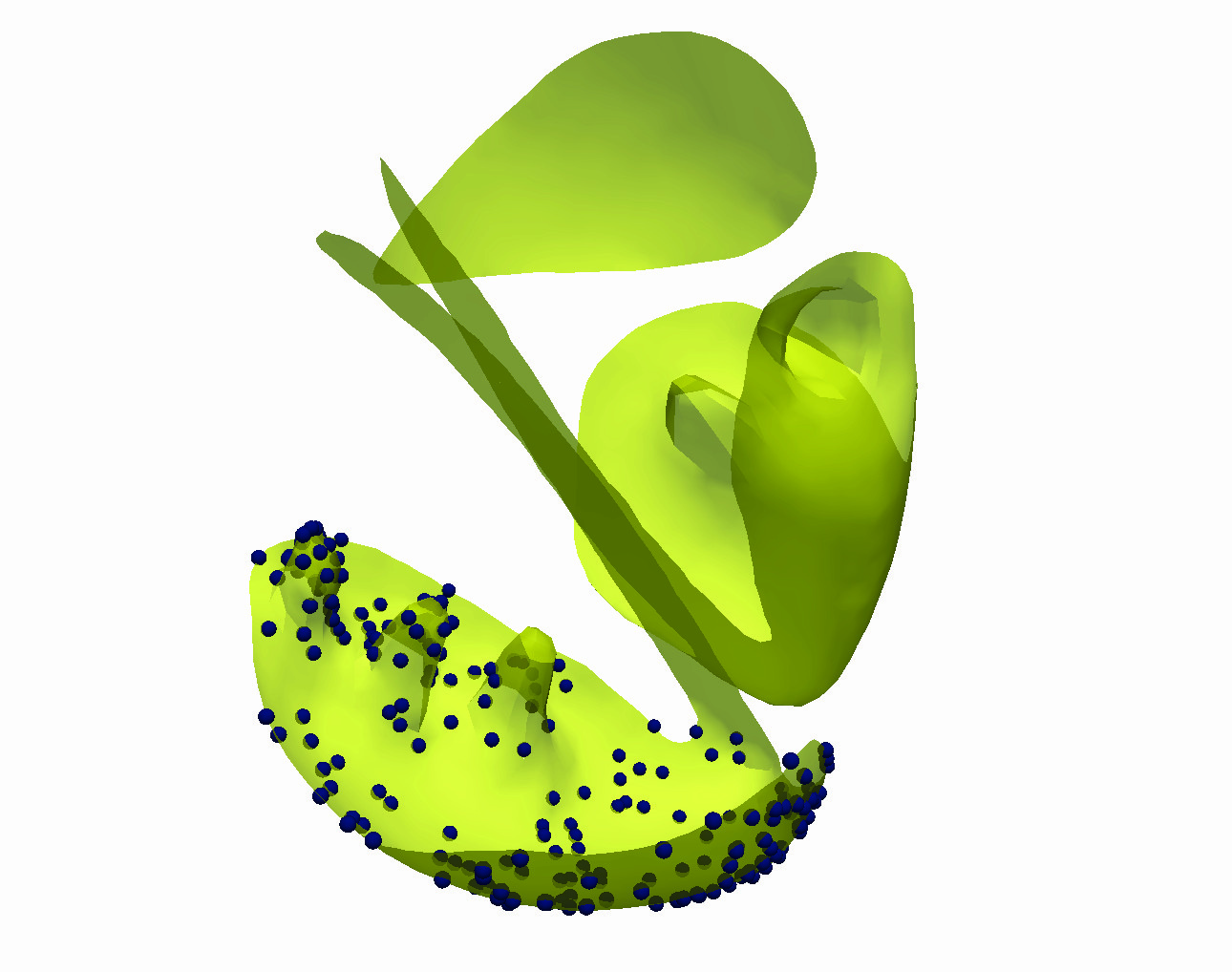
As sketched in Figure 9, the communication between the 1D mesh and the underlying 2D (or 3D) counterpart occurs through some communication nodes (CNs, indicated by red circles) which are defined in the preprocessing phase as a subset of the bundle grid nodes (black dots). In particular, as the trans- membrane potential at a CN exceeds a certain threshold (here set to 0 mV), an external localized stimulus Is (with Sa = 1 mA/mm2 and Sd = 0.5 ms, see equation (4)) is applied to the underlying 2D (or 3D) mesh cells within a distance RS from the CN, thus initiating a depolarization front in the 2D (or 3D) media. Specifically, since the 1D domain represents the network of intern- odal pathways that are some millimeters thick in the atrial myocardium , the communication range for the coupling between the 1D and the 3D atrial mesh is taken equal to RS = 1 mm, whereas any CNs between the 1D and the 3D ventricular mesh are not present since the bundles do not directly excite the ventricular myocardium (they are isolated by fibrous sheaths) but they only transfer the propagation front to the Purkinje network . Hence, the depo- larization of the Purkinje mesh is initiated by the CNs between the 1D and the 2D domains having a smaller communication range of RS = 0.1 mm, scaling as the local Purkinje thickness. Although all bundle nodes (black dots in Fig- ure 9) can be taken as CNs, only a subset of them is used in order to reduce the computational cost of the coupling since at any timestep the local trans- membrane potential at the CNs should be monitored for eventually applying a localized electrical stimulus. In this work, the CNs are equally distributed over the 1D network with a relative distance among them of ς · τ ≈1 mm, where ς = 2 m/s is the typical internodal pathways propagation speed and τ = 0.5 ms is the maximum time delay in the activation between two consecutive CNs. As

20

a consequence, a shorter τ would correspond to a denser distribution of the CNs and vice–versa.

Sparse Connection

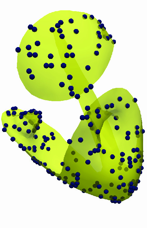
Figure 10: Distribution of the communication nodes (CNs) between the 2D Purkinje and the 3D ventricular myocardium, corresponding to the Purkinje muscle junctions (PMJs). Figure 10 show the distribution of the CNs between the 2D and the 3D ven- tricular media (RS = 0.1 mm), which allow the Purkinje network to activate the ventricular myocardium with an orthodromic delay of 5 milliseconds . The density and the positions of these CNs is user–defined and it has been set so to reproduce the ones of the Purkinje muscle junctions (PMJ) [60, 73]. In this work 300 CNs equally distributed among the left and right ventricles have been considered with their distribution corresponding to the one of the PMJ with no CNs present in the interventricular septum as the Purkinje network is insulated by fibrous sheaths in that region [75, 72] (Figure 10 a).

In the case of healthy cardiac electrophysiology, the electrical coupling through the CNs is one–way, meaning that only the lower topological domain triggers an electrical stimulus on the higher one, e.g.

The 1D Bundle Excites The 3D

myocardium but not vice–versa. On the other hand, in some pathological cases such as nodal re-entry tachycardia or antidromic propagation (re–enter of the signal in the Purkinje network from the myocardium) , the coupling is

21

two–way and the 3D myocardium can eventually excite back the 1D bundles and the 2D Purkinje, as shown in § 5.

Δx=0.2 Mm, Δt=0.05 Ms

Figure 11: Activation time along the main diagonal in the a) 1D, b) 2D and c) 3D domain according to the monodomain model for various temporal and spatial resolutions (∆x is the grid spacing the x direction in 1D, x, y in 2D and x, y, z in 3D). The corresponding average transmembrane potential is reported in d), e) and f), respectively.

The convergence of the numerical method is investigated using a procedure similar to the one reported in the benchmark paper by solving the mon- odomain and the bidomain equations over a 3D cartesian domain of size 20×7×3 mm3 coupled with the ten Tusscher–Panfilov cellular model . In order to val- idate the 2D and 1D solvers, a similar test–case is also run on a rectangular 2D domain (20 × 7 mm2) and on a straight linear domain (of length 20 mm). In all cases, the domain is discretized with a uniform spatial grid with grid size of

Δx=0.1 Mm, Δt=0.05 Ms

Figure 12: Same as Figure 11 but solving the bidomain electrophysiology model. 0.5, 0.2 and 0.1 mm in each direction (x in the 1D, x, y in the 2D and x, y, z in the 3D), and three different timesteps have been used, namely 0.05, 0.01 and 0.005 ms. The muscle fibers are taken aligned with the long axis direction (20 mm in 2D and 3D) and the electrophysiology parameters, including the initial state variables of the cell model, are set as in . The initial stimulus is ap- plied within a line/square/cube of side 1.5 mm placed in the corner closer to the origin.

In the case of the monodomain solver, Figure 11 reports the activation time (defined as the instant when the transmembrane potential exceeds 0 mV) along the diagonal of the domain departing from the corner where the stimulus is applied for the (a) 1D (b) 2D and (c) 3D domains. The corresponding trans- membrane potential averaged in the domain volume V , v(t) =

V V(X, T)Dv/V

are reported as a function of time in Figure 11(d,e,f), showing that, as the spa- tial grid is refined, the propagation speed of the depolarization front increases

23

until convergence is attained for the more refined grid spacing with a timestep equal–smaller than ∆t = 0.01 ms. The corresponding convergence curve for the bidomain model are given in Figure 12 for each topological dimension of the conductive media, thus showing similar results for the same grid spacing and timestep.

Δx=0.1 Mm, Δt=0.005 Ms

Figure 13: Average transmembrane potential in the 3D domain according to a) the mon- odomain and b) the bidomain electrophysiology model.

A) Our Numerical Results (Yellow

dashed line for ∆x = 0.2 mm and red dashed one for ∆x = 0.1 mm) are compared against the average results (blue solid line) of the benchmark paper , where the shaded area indicates the corresponding standard deviation. In panel b) our code is validated against the results reported .

In the 3D case, the numerical solution of the monodomain and bidomain equations can be validated against previous results from the literature. The for- mer is validated against the benchmark paper of Niederer et al. 2011 where 11 different numerical codes (either based on finite elements or finite differences) have been used and the resulting average activation time along the diagonal of the cubic domain (blue solid line) and standard deviation (blue shaded region) are reported in Figure 13 (a). Moreover, the solution of the bidomain equations is validated against the results of Cuccuru et al. , which is reported in Fig- ure 13 (b) for different spatial steps and different polynomial degrees, see

24

for further details on their numerical method. Both the monodomain and the bidomain results obtained with our numerical solver fit well those reported in the literature.

1D Ab

Figure 14: (a) Spatial and (b) temporal numerical accuracy of the 1D, 2D, and 3D mon- odomain solver. In (a) the error on the average transmembrane potential (computed at time t = 50 ms for ∆t = 0.005 ms) is shown as a function of the mean grid size, ∆x. In (b) the same quantity (at time t = 50 ms for ∆x = 0.31 mm) is reported as a function of the timestep, ∆t.

The corresponding numerical accuracy of the solver is reported in Figure 14 in the case of the 1D, 2D and 3D monodomain model. Figure 14(a) indicates the second order spatial accuracy of the FV method by showing the error on the average transmembrane potential over the domain at time t = 50 ms (and timestep set to ∆t = 0.005 ms) as a function of the average grid size, ∆x.

On the other hand, Figure 14(b) reports the same quantity (evaluated with ∆x = 0.31 mm) as a function of the timestep ∆t, thus retrieving the first order temporal accuracy of the Rush–Larsen temporal integration scheme, where the non–gating variables are solved using forward Euler. The numerical error could be reduced by adopting a second–order Adams–Bashforth scheme for the non– gating variables (dashed blue line for the 1D case), although a modified second order Rush–Larsen scheme would be needed to attain a second order accu-

25

racy.

Cpu

monod.

Gpu

monod.

Speedup

monod.

177

Table 1: Wall–clock time for integrating a single bidomain and monodomain time step for the three Cartesian grids considered in Figures 11–13. The CPU time is obtained using a single core Intel(R) Xeon(R) Gold 6230 with 2.10GHz, whereas the GPU time corresponds to a Tesla V100 from Nvidia.

Table 1 reports the wall–clock time for solving a single bidomain and mon- odomain timestep on the benchmark Cartesian domain using a single CPU core or GPU device. Running the GPU version of the code yields a significant speedup in all cases, which increases as the grid gets more refined owing to the better balance of workload across the GPU threads running in parallel. It can be observed, that the speedup is larger in the case of monodomain computations with respect to the bidomain counterpart because the Arnoldi iteration and the solution of the corresponding Hessenberg system in the GMRES algorithm are based on the Lapack library running on the CPU.

The convergence of the numerical solution over the cardiac domains used in sections 2 and 5 for the electrical conductivities reported in Table 2 is assessed by monitoring the average transmembrane potential as a function of time, v(t).

Figure 15(a) shows v(t) solved over the 1D network of fast conduction bundles using the monodomain model coupled with the Courtemanche cellular model with a timestep equal to ∆t = 0.001 ms, thus showing good convergence for a spatial discretization finer than ∆x = 0.25 mm (corresponding to a number of cells equal to 2′000). On the other hand, the monodomain equations over the right Purkinje 2D media coupled with the Stewart cellular model are at

Related Journal Articles & DOI Links

Selected peer-reviewed publications relevant to 12 Lead ECG Acquisition. Click the DOI to access the full paper (may require institutional access).

Why Choose Us?

Bangalore guidance for robotics, Spectre and autonomous systems projects.