Simulia Tosca Structure Optimization

Optimal Design of Frame Structures with Mixed Categorical and Continuous Design Variables Using the Gumbel-Softmax Method∗ Mehran Ebrahimi†,a, Hyunmin Cheonga, Pradeep Kumar Jayaramana, and Farhad Javida

Abstract

In optimizing real-world structures, due to fabrication or budgetary restraints, the design vari- ables may be restricted to a set of standard engineering choices. Such variables, commonly called categorical variables, are discrete and unordered in essence, precluding the utilization of gradient-based optimizers for the problems containing them. In this paper, incorporating the Gumbel-Softmax (GSM) method, we propose a new gradient-based optimizer for handling such variables in the optimal design of large-scale frame structures. The GSM method provides a means to draw differentiable samples from categorical distributions, thereby enabling sensitivity analysis for the variables generated from such distributions. The sensitivity information can greatly reduce the computational cost of traversing high-dimensional and discrete design spaces in comparison to employing gradient-free optimization methods. In addition, since the developed optimizer is gradient-based, it can naturally handle the simultaneous optimization of categorical and continuous design variables. Through three numerical case studies, different aspects of the proposed optimizer are studied and its advantages over population-based optimizers, specifically a genetic algorithm, are demonstrated.

Keywords Categorical design variables, Gumbel-Softmax method, Frame structures, Structural optimization, Differentiable sampling, Sensitivity analysis

Introduction

The application of frame structures composed of interconnected beams and columns is ubiquitous in various fields of engineering making their simulation and optimization attractive subjects of interest in both academia and industry . Commonly, the finite element (FE) analysis of frame structures is performed by modeling their components with beam elements which are capable of undergoing longitudinal (axial), transverse (bending) and torsional deformations, unlike truss ∗This is a preprint of an article published in Structural and Multidisciplinary Optimization. The final authenticated version is available online at: https://doi.org/10.1007/s00158-024-03745-7.

Arxiv:2501.00258V1 [Cs.Ce] 31 Dec 2024

elements that can handle only the first one. Accurately capturing these deformation modes and their interactions makes the simulation of frame structures computationally more demanding than that for truss structures . The difference becomes particularly more noticeable and exceedingly cumbersome in the optimal design of large-scale frame structures which has led to considerably fewer extensive investigations of this topic for such structures in the literature.

The focus of the present paper is the optimal design of frame structures with mixed categorical and continuous design variables. Categorical design variables are inherently discrete and their values belong to an unordered set of available choices. Examples of such variables in frame structures include beam cross-sections (profiles) and materials.

In Real-World Applications, Only A Limited

number of cross-sectional profiles and material choices may be available to design a structure due to various limitations such as manufacturing process and cost. For instance, the beam material may only be steel or aluminum, and its cross-section may only be I-profile or T-profile with limited options for their geometrical attributes. Therefore, for practical purposes, it is crucial to distinguish between categorical and continuous design variables, as the latter ones are free to take any value within their bounds and are more straightforward to handle.

The challenges associated with considering categorical design variables are not exclusive to frame structures and have been explored significantly in other application areas .

Of Particular

relevance to this paper are truss structures and the techniques developed for handling categorical variables therein. A worthwhile review of the available techniques for truss structures can be found in . Although frame and truss structures behave differently, they bear a close resemblance in the way they are designed. Thus, the methodology and arguments presented in this paper are directly applicable to truss structures as well.

Broadly, existing optimization techniques applied to structural problems with categorical variables can be classified into gradient-free and gradient-based schemes. The majority of methods developed for these problems utilize gradient-free optimizers such as the branch-and-bound [2, 11], genetic algorithm (GA) , simulated annealing and particle swarm optimization , among others. It is well-known that due to the combinatorial nature of problems with categorical design variables, the computational cost associated with exploring their design space, which typically grows exponentially with the number of variables, becomes intractable for large-scale problems using the gradient-free optimization routines . Hence, most cases studied in the literature involve structures with a small number of components and a few (predominantly two) categorical choices per element (component).

Employing gradient-based optimization techniques can be considered as a remedy to alleviate the scalability issue . However, as the categorical variables are discrete and more importantly unordered, computing the gradients of objective and constraint functions with respect to these variables is problematic. There are hence rare precedents of incorporating gradient-based optimiz- ers in the optimal design of beam and truss structures with categorical design variables .

The proposals in this area apply some form of approximation to compute the function gradients with respect to the categorical variables (e.g., relaxation of discrete to continuous variables , which only makes sense if the variables are ordered) along with rounding techniques to enforce the discreteness of the categorical variables. In another body of work [22, 24], the weights associated

2

with each categorical choice, in their case material types, are treated as design variables. Subse- quently, in the Heaviside function has been applied to penalize the intermediate weight values to a particular categorical choice.

One can think of several scenarios where these approaches fall short and a more robust technique is desired. For instance, if cross-sectional profiles are design variables in a problem, say I-, T- and U-profiles, it is mathematically challenging (if not impossible) to interpret the meaning of the gradient of a function with respect to these profiles in a direct sense. One possible solution to this problem is to work with the attributes of categorical variables. For example, instead of operating directly on the cross-sectional profiles, their areas can be taken as design variables.

However, this becomes troublesome when categorical variables have multiple attributes influencing the optimization progress in a conflicting manner, such as for a cantilever beam under gravity where its cross-sectional area and its second moment of area can affect the beam’s deflection in opposing ways. Furthermore, relaxing the discrete variables to continuous ones—inspired by the SIMP method for the topology optimization of solid structures —is often limited to problems wherein categorical variables are ordered or have only two choices.

In this paper, we propose a technique for resolving the aforementioned issues in computing the gradients with respect to categorical variables, thus enabling the use of gradient-based optimizers in structural design problems. This novel optimization scheme is founded upon two main ideas.

Firstly, we propose reparametrizing the categorical design variables and taking the probability of using them in the structure as their corresponding design variables. For instance, if a categorical variable is a beam’s cross-section chosen from I-, T- and U-profiles, we propose taking the prob- abilities of having I-, T- and U-profiles for that beam as its corresponding design variables. As a result, instead of discrete variables, the optimizer deals with continuous ones. Consequently, the optimization functions must be reparameterized in terms of the probabilities and their sensitivity analysis must be carried out with respect to these probabilities, the details of which are presented in the forthcoming sections. Obviously, defining functions in terms of probabilities makes them probabilistic (i.e., stochastic) and in order to compute their values a sampling process is involved, which is in general nondifferentiable. Therefore, secondly, we propose using the Gumbel-Softmax (GSM) technique for making the sampling process differentiable .

The GSM method is a relaxed version of the original Gumbel-Max (GM) method that provides a simple mechanism for drawing differentiable samples from a categorical probability distribution parameterized by the unnormalized log-probabilities of the classes (choices) of that categorical variable . In recent years, since the seminal papers and , the GSM method and its variants have garnered significant attention in the machine learning community (e.g., ).

The intrinsic commonalities between combinatorial problems in machine learning and (structural) engineering applications prompted us to explore the utilization of the GSM technique in frame structures. To the best of the authors’ knowledge, this study is the first of its kind to employ the GSM method in optimization problems involving mixed continuous and categorical design variables.

The remainder of the present paper is organized as follows.

Section 2 Introduces The General

problem formulation and the notations involved. In Section 3, we present the GSM method; the pivotal ingredient of the proposed optimization technique in this study. Then, in Section 4, the

3

details of the optimizer are laid out. Three numerical examples are provided in Section 5 to assess the performance of the developed optimizer and discuss its various aspects. Finally, the paper is concluded by making a few remarks about our proposal in this article and potential considerations for further improvement.

Problem Statement

The optimal design problem of a frame structure can be posed as follows. Given a frame struc- ture, find the optimum values of continuous design variables as well as optimum choices for the categorical design variables such that the target structural performance function is achieved and the governing linear elasticity equations due to a FE discretization and imposed constraints are satisfied. Accordingly, the topology of the structure does not change throughout the optimization routine. Denoting x := [x1, · · · , xnx]T and c := [c1, · · · , cnc]T as the vectors of continuous and categorical design variables, respectively, the optimization problem mathematically reads

Ci ∈{1, · · · , Ni},

i = 1, · · · , nc. In this equation, J is the scalar-valued objective function, g ∈Rng represents the vector of op- timization constraint functions, K ∈Rnu×nu indicates the structure’s stiffness matrix, f ∈Rnu specifies the external load vector, and u ∈Rnu denotes the vector of nodal displacements (state variables). Also, lbi and ubi, i = 1, · · · , nx, refer to the lower and upper bounds of the continuous variable xi, respectively. Furthermore, Ni, i = 1, · · · , nc, is the number of choices available for the categorical variable ci. Therefore, without loss of generality, we assume the existing choices for each ci, i = 1, · · · , nc, are indexed as {1, · · · , Ni}.

Depending on the problem at hand and the capabilities of the FE solver, J and g can be linear or nonlinear functions of their arguments. Other than continuity and (at least first order) differen- tiability, we make no further assumptions on J and g. Given a structure, some examples of these functions include mass, compliance, displacement, von Mises stress and natural frequencies. Since the response of a structure is affected by the values of the design variables, the nodal displacements u are implicit functions of x and c. As mentioned in the introduction, we aim to use gradient-based optimizers to solve the problem in (1). However, due to the challenges elaborated earlier, direct

4

computation of ∇c J and ∇c g gives rise to mathematical hurdles. Thus, we restate (1) as

I = 1, · · · , Nx,

where θ := [θ1,1, · · · , θ1,N1, θ2,1, · · · , θ2,N2, · · · , θnc,1, · · · , θnc,Nnc]T denotes the vector of unnormal- ized log-probabilities of the categorical variables formulated in (3). The first and second indices in θi,j refer, respectively, to the variable index and its available choices’ index. If for a categorical vari- able i, the probability of using its Ni choices in the structure is defined by pi := [pi,1, · · · , pi,Ni]T ,

(3)

where pi,j is the likelihood of choice j for categorical variable i. Here, we opt for using unnor- malized log-probabilities θi,j, i = 1, · · · , nc, j = 1, · · · , Ni, as the design variables instead of their corresponding probabilities pi,j. Once the optimal values of θi,j’s are found, their corresponding optimal probabilities pi,j can be computed through the Softmax function as

,

i = 1, · · · , nc, j = 1, · · · , Ni.

(4)

The benefits of using θi,js are twofold. Firstly, following (3), as opposed to pi,js that are between 0 and 1, unnormalized log-probabilities θi,js are unbounded continuous variables and can take any value between −∞and +∞. Secondly, for each categorical variable i the probabilities must

Satisfy Pni

j=1 pi,j = 1 at each optimization iteration, whereas working with its associated θi,js and eventually converting them to pi,js using (4) would naturally satisfy this constraint. This reduces the number of optimization constraints significantly, especially in large-scale problems.

In order to utilize gradient-based optimizers, one needs to compute the sensitivities (gradients) of objective and constraint functions with respect to θ and x (i.e., ∇xJ, ∇xg, ∇θJ and ∇θg). Most often, in structural engineering problems, J and g are not explicit functions of the probabilities θ.

For instance, for a categorical variable corresponding to a beam’s material, J and g are functions of the properties of the selected material such as its Young’s modulus or density, not the material itself as an object. Therefore, for all categorical variables, a sampling process must be performed independently to draw a sample from each of their existing choices based on their probabilities and then compute the values of J and g using that sample. The sampling process, however, in general breaks down the differentiability of these functions. This issue can be resolved by incorporating the GSM method. In the subsequent section, the GSM method and its application in having a differentiable sampling procedure are introduced.

Differentiable Sampling Via The Gsm Method

For conciseness, the subject of the current section is presented only for J. The same idea can be directly applied to the constraint functions g in a similar fashion. The goal is to compute the value of J and its gradient with respect to the vector of unnormalized log-probabilities θ. For the sake of brevity, we assume θ is associated with just one categorical variable with N choices and J is only a function of θ (and not x and u as in the previous section). More general cases are provided in Section 4. Note that J is not an explicit function of θ but rather the continuous attributes (properties) of a sample (i.e., choice) drawn from the categorical distribution function characterized by θ. In other words, once a sample is picked from the categorical distribution of θ, the value of J using the properties of this sample is computed.

A categorical distribution function is a discrete probability distribution specifying the likelihood of the choices (classes) for a categorical random variable .

For Instance, Applying (4), The

categorical distribution of θ is pθ := {(softmax(θ))1, · · · , (softmax(θ))N}. A one-hot sample vector s can be generated from pθ utilizing Algorithm 1. The size of s is N and its entries are all 0 except for the index corresponding to the selected class at which its entry is 1. Suppose the attributes of the selected class are collected in a vector a. Since J is a function of θ through the drawn sample and its attributes, it can be formulated as J (a (s(θ))). The sensitivity of J with respect to θ

Therefore Can Be Written As

∇θJ = (∇θa)T ∇aJ = (∇sa ∇θs)T ∇aJ.

(5)

The sample vector s, generated by incorporating the common sampling process described in Algo- rithm 1, is not differentiable with respect to θ creating issues in computing ∇θs and consequently ∇θJ in (5). The step causing nondifferentiability is Step 5. The GSM method resolves this issue by a simple yet remarkably efficient solution .

The Gsm Method

We first introduce the GM method from which the GSM method is derived (recall that GM stands for Gumbel-Max). Define I(i) as an operator that returns a one-hot vector of size N with an entry of 1 at index i and zero elsewhere. In the GM method, a sample vector s is generated by

(6)

where θi, i = 1, · · · , N, are unnormalized log-probabilities of the classes and G(i), i = 1, · · · , N, are independent and identically distributed samples (noises) generated from the standard Gumbel distribution Gumbel(0, 1). For each class index i, the noise G(i) can be obtained by independently sampling Gumbel(0, 1) through drawing a uniformly distributed random real number r and setting G(i) = −ln (−ln(r)) . Therefore, instead of employing Algorithm 1, which is the common, nondifferentiable way of drawing samples from a categorical distribution, s can be drawn from θ

6

Algorithm 1: The common, nondifferentiable way of drawing samples from a categorical

Distribution

Input: Unnormalized log-probabilities θ ∈RN associated with a categorical variable. Output: One-hot sample vector s.

1 Initialize S ∈Rn By Zeros;

2 Compute the probabilities pi, i = 1, · · · , N, using (4) and put them into a (not necessarily

Ordered) Set Pθ := {P1, · · · , Pn};

3 Calculate the corresponding cumulative distribution function as

Pi};

4 Choose a uniformly distributed random real number r ∈[0, 1]; 5 Find the largest index i in pθ such that (pθ)i ≤r; 6 Set the entry in s corresponding to index i to 1; by perturbing each entry of θ via independently adding a Gumbel noise to them, selecting the index corresponding to the largest perturbed entry of θ, and returning the sample associated with that index. The sample vector s produced this way has theoretically the same distribution as the categorical distribution associated with θ (i.e., s ∼pθ). For the sake of conciseness, the proof of this statement is provided in Appendix A. It is of the utmost importance to note that in (6) only the noise generated from the standard Gumbel distribution—and not any other types of probability distributions—results in a sample vector s ∼pθ. Interested readers may refer to [27, 29, 30] for further details about the GM method and other versions of the proof.

Since the arg max function in (6) is not differentiable, Jang et al. proposed a continuous, differentiable approximation (relaxation) to this function by introducing a temperature parameter τ and utilizing a so-called soft one-hot sample vector es with entries

(7)

or put it shortly es = softmax ((θ + G)/τ) with G := [G(1), · · · , G(N)]T . Although esi entries in (7) have the advantage of being differentiable with respect to θi, i = 1, · · · , N, there are two concerns with having a soft one-hot sample vector es in the GSM method.

Firstly, Due To The Applied

relaxation, es does not exactly follow the pθ distribution, as opposed to s in (6). However, as τ →0, this soft one-hot vector becomes a true one-hot vector and subsequently, the samples generated by the GSM method would have the exact pθ distribution . Therefore, at the beginning of the optimization routine, one can set τ to a high temperature (in a relative sense) and using an annealing scheme reduce it to a small nonzero value as the optimization progresses. For machine learning applications, the typical range suggested for τ is between 100 to 0.1 (e.g., [33, 37–39]).

More details about the annealing scheme and temperature range used in this study are provided

7

in Section 5. Secondly, with regard to the concerns facing the GSM method, having a soft one-hot vector es leads to generating a sample vector that is a combination of all choices in the target categorical variable which oftentimes does not bear any physical realization, causing problems in computing the value of J and its gradients. For example, for the applications considered in this paper, we cannot have a beam cross-sectional profile that is a combination of I- and U-profiles. In such scenarios, the so-called straight-through GSM can be adopted to generate a true one-hot sample vector

(8)

and to compute the value of J using this vector. Then, for the sensitivity analysis in (5), since bs is not differentiable with respect to θ, ∇θes instead of ∇θbs is utilized.

As The Optimization

advances and es approaches toward being a true one-hot vector, the discrepancy between ∇θes and ∇θbs diminishes. Ultimately, following (5) and generating es using the GSM method, the gradient

(10)

is easily derived using (7). Note that although G(i), i = 1, · · · , N, which are random Gumbel noises appear in computing esi values in (7), they do not cause any differentiability issues in (9) and (10). Assuming ∇aJ and ∇esa are known, Algorithm 2 encapsulates the steps involved in the GSM method for generating sample vectors es and bs, as well as computing the value of a function J that through es is implicitly a function of unnormalized log-probabilities θ corresponding to a categorical distribution and eventually calculating ∇θJ. The details of computing ∇aJ and ∇esa are laid out in the next section.

Optimization Methodology

In Section 3, the GSM method was described in its most general form regardless of the application. Henceforth, to establish a more oriented dialogue, we limit the scope to structural problems and optimization functions arising in such applications. Considering the optimization problem stated in (2), in this section, we develop a scheme to compute the sensitivities of the optimization objective and constraint functions (J and g, respectively) with respect to both x and θ. Without loss of generality, we only focus on computing ∇xJ and ∇θJ. Computing ∇xg and ∇θg proceeds similarly.

For the structural problems considered in this article, continuous design variables x could be compo- nents’ cross-sectional dimensions (or properties), their orientation, length and material properties.

8

Algorithm 2: The GSM method for computing the value and gradient of a function of a

Categorical Distribution

Input: Function J and its gradients ∇aJ and ∇esa, unnormalized log-probabilities θ ∈RN associated with a categorical variable, temperature parameter τ. Output: J and ∇θ J.

1 Generate samples G(i), i = 1, · · · , N, from the standard Gumbel distribution Gumbel(0, 1);

4 Get J Using Bs;

5 Compute ∂esi/∂θj, i, j = 1, · · · , N, using (10);

6 Get ∇Θ J Via (9);

The categorical variables may be material and cross-sectional profile choices of each component. The categorical variables are determined by their corresponding continuous attributes. For example, material choices are characterized through their Young’s modulus, Poisson’s ratio and density. The objective and constraint functions may be the structure’s mass, its compliance, nodal displacement and maximum stress to name a few. The proposed optimization framework and required deriva- tions are elucidated in a general format such that other types of design variables and functions can be incorporated in a straightforward manner.

For the sake of brevity, suppose the aim is to compute the sensitivities of J with respect to a single continuous variable xl, l = 1, · · · , nx and unnormalized log-probabilities θm := [θm,1, · · · , θm,Nm]T associated with a single categorical variable cm, m = 1, · · · , nc. Subsections 4.1 and 4.2 present the procedures for computing ∇xlJ and ∇θmJ, respectively. Once sensitivities of J are calculated, they can be utilized for optimizing the frame structures using the optimization approach proposed in Subsection 4.3.

Sensitivity Analysis For Continuous Variables

Recall from Section 2 that J can explicitly and implicitly be a function of xl (and θm) through u. Accordingly, the gradient of J with respect to xl is expressed as

(11)

where ∂J/∂xl and ∇uJ which are, respectively, explicit derivatives of J with respect to xl and u can be carried out in a simple manner knowing the function formulation, thus not further elaborated in this paper. For example, if J = 0.5uT Ku, then ∂J/∂xl = 0.5uT (∇xlK) u and ∇uJ = Ku. The onerous term in (11) is ∇uJ for which we appeal to the adjoint method well-known to be advantageous over the direct differentiation method for optimizing problems with several design variables. The process is presented for a general J that may be a linear or nonlinear function of its arguments. Using the discretized governing equation Ku −f = 0 and differentiating it with

(12)

where it is assumed that the external force vector f is only a function of xl not u. Since the left-hand side of (12) is zero, multiplying it by any arbitrary vector of a conforming size to the governing equation also results in zero. Denote this multiplier vector, called the adjoint variable vector, by λJ ∈Rnu. Applying it to (12) and employing the result in (11) leads to

+ ∇Xlu · ∇Uj −Λj · (K ∇Xlu + (∇Xlk) U −∇Xlf) ,

l = 1, · · · , nx.

(13)

This equation holds regardless of the value of λJ; ergo, it can be chosen such that ∇xlu in (13)

Vanishes. Meaning

KλJ = ∇uJ.

(14)

Once λJ is found through (14), putting it in (13) gives

−Λj · ((∇Xlk) U −∇Xlf) ,

l = 1, · · · , nx.

(15)

This is the final equation for computing the sensitivity of J with respect to continuous design variables. Note that solving (14) can be carried out quite efficiently as factorizing K, the arduous step in the solution process, has already been performed in solving the governing equation Ku = f.

Furthermore, there is no dependence on xl or any other continuous design variable in (14); hence (14) is solved only once (and not for each variable individually), justifying the application of the adjoint method for problems with several design variables. The adjoint equation for each constraint

Function Gi, I = 1, · · · , Ng, Is Formulated As

Kλgi = ∇ugi.

Sensitivity Analysis For Categorical Variables

With respect to θm, the gradient of J using (5) reads ∇θmJ = (∇esma ∇θmesm)T ∇aJ = ∇aJ · (∇esma ∇θmesm) ,

(17)

where esm is the sample vector drawn from the categorical probability distribution characterized by θm employing the GSM method. Calculating ∇θmesm can be performed incorporating the procedure developed in Section 3 and (10). We first focus on handling ∇esma and then ∇aJ in (17). Naturally, each entry of esm corresponds to a class which can be characterized by some continuous attributes (properties). If esm is associated with an isotropic material its entries are determined by Young’s modulus and Poisson’s ratio. On the other hand, if esm is linked to a cross-sectional profile, the relevant continuous attributes are cross-sectional properties such as area and second moments of area. It is important to note that all the choices considered for a categorical variable must be characterized using the same set of attributes.

10

Suppose esm corresponds to a categorical variable with Nm choices. Let ak := [a1,k, · · · , anm,k]T , k = 1, · · · , Nm, be the vector of size nm containing the continuous attributes of each choice. Also, define Am ∈Rnm×Nm the attribute matrix of this categorical variable as

A1,Nm

... ... ...



.

(18)

If esm is a hard one-hot vector, the attributes of the selected class in this categorical variable can

Be Picked Out By

a = Amesm.

(19)

As mentioned earlier in Section 3, for running the structural simulation and computing the opti- mization functions, bsm (given by (8)) instead of esm needs to be used in (19). During the sensitivity analysis, however, esm itself is employed leading to ∇esma = Am. As the optimization advances, esm approaches bsm. Finally, inserting this relation into (17) yields

∇Θmj = ∇Aj · (∇Esma ∇Θmesm) = ∇Aj · (Am ∇Θmesm) ,

m = 1, · · · , nc.

(20)

In this equation, ∇aJ is the sensitivity of J with respect to the a associated with the continu- ous attributes of the class with the highest unnormalized log-probability at a given optimization iteration (i.e., the attributes of the sample generated by the straight-through GSM). Since a is a continuous variable, computing ∇aJ can be carried out by adopting the adjoint method described

(21)

with the same λJ found by (14). Equation (20) is the final equation for computing the sensitivity of J with respect to θm. To further clarify the presented procedure for computing ∇θmJ, we provide the following example. Suppose an optimization problem whose categorical design variables are the cross-sectional profiles of its beams. Assume for one of the variables the choices are circular and rectangular profiles each characterized by their area A, second moments of area Iyy and Izz and torsion constant K. Also, let θ = [θ1, θ2]T be the unnormalized log-probabilities associated with each profile at a given optimization iteration. For this variable, the attribute matrix A reads



.

(22)

There may be two scenarios for θ1 and θ2 at any optimization iteration: 1. θ1 ≥θ2: leading to es1 ≥es2 using (7) and bs = [1, 0]T according to (8).

11

2. θ1 < θ2: resulting in es1 < es2 based on (7) and bs = [0, 1]T utilizing (8). In the former situation, J and ∇aJ in (20) are computed employing the circular profile and its continuous attributes, otherwise, the rectangular profile is adopted.

Finally, ∇Θj Is Obtained

through ∇esma = A, finding ∇aJ via (21) and calculating ∇θes applying the GSM method. We once again highlight that as the optimization moves toward convergence, es approaches a true one- hot vector and the errors due to the applied relaxations inherent in the GSM method dwindle.

Optimization Scheme

The proposed optimization routine—named GSMO standing for Gumbel-Softmax optimization— for frame (or truss) structures with mixed categorical and continuous design variables is presented in Algorithm 3. Although this scheme is described for a particular class of structures undergoing linear elasticity behavior, it can be applied with minor modifications to other problems (not necessarily structural) with mixed categorical and continuous design variables governed by a different set of physics equations.

An important fact about GSMO in Algorithm 3 is that there is no stratification between continuous and categorical design variables. In other words, both classes of variables are handled concurrently in each optimization iteration, thus giving no priority to either of them. This is unlike the bilevel optimization routines where categorical and continuous variables are treated at different levels (stages) . In such techniques, first, the categorical variables are taken into account and the structure is optimized updating only those. Then, in the second level, the continuous design variables are handled. A shortcoming of these approaches is that each variable type is optimized sequentially at one level at a time, which may lead to underperformance. Nevertheless, a bilevel version of GSMO, named BiGSMO, is provided in Algorithm 4 of Appendix B and assayed against GSMO in the forthcoming section.

Case Studies

Prior to introducing the case studies, we note a few remarks. Since the GSM method relies on generating Gumbel samples which is a stochastic process, the optimum solution found through GSMO (and BiGSMO) may vary every time the optimization is executed. Therefore, GSMO (and BiGSMO) shares a similarity in this aspect with stochastic optimizers such as GA. Hence, to make a fair comparison with stochastic methods, we run each of the case studies 10 times and report the best, average and standard deviation of optimum solutions. As for the temperature τ in (7) and its annealing scheme, an initial temperature of 100 scaled by 0.9 per iteration is adopted. The minimum temperature is kept at 0.01. Other options for the temperature and its annealing scheme are described in . Also, a step size of 10−3 is set for the optimization routine. These choices can be seen as hyper-parameters for GSMO. Moreover, an identical initial probability value is assigned to the available choices of each categorical variable. Further remarks about them are provided in the conclusion section.

12

Algorithm 3: The GSMO scheme for optimizing frame/truss structures with mixed cat-

Egorical And Continuous Design Variables

Input: Objective function J, constraint functions g, continuous design variables x and their bounds, categorical design variables c and their available choices, GSM annealing scheme.

Output: Optimum design.

1 Initialize X;

2 Initialize θi, i = 1, · · · , nc, for each categorical variable ci by entry values of zero assuming

5

Generate Gumbel noises G(j), j = 1, · · · , Ni, from the standard Gumbel

6

Compute (esi)j, j = 1, · · · , Ni, using (7) and ∇θiesi via (10);

9

Solve the governing equations Ku = f using bsi, i = 1, · · · , nc, and get u;

10

Compute J and g values using bsi, i = 1, · · · , nc, and u;

12

Compute ∇ugi, i = 1, · · · , ng, then find λgi, i = 1, · · · , ng, by solving (16);

13

Calculate ∂J/∂xi, ∂g/∂xi, ∂K/∂xi and ∂f/∂xi, i = 1, · · · , nx;

14

Get ∇xJ and ∇xg incorporating the corresponding adjoint vectors and (15);

17

Calculate ∂J/∂ai, ∂g/∂ai, ∂K/∂ai and ∂f/∂ai using the attributes of the selected

18

Compute ∇aiJ and ∇aig utilizing the adjoint vectors found in Steps 11 and 12,

21

Update x and θi, i = 1, · · · , nc, using the sensitivities found in Steps 14 and 19;

22 End

Unfortunately, the relevant literature to this article lacks a repository of well-documented bench- marks, particularly for beam structures . Nevertheless, to study the performance of GSMO, its results are compared to those reported in using different optimization techniques (which includes GA, particle swarm optimization (PSO) , mine blast optimization (MBO) , wa- ter cycle optimization (WCO) , colliding bodies optimization (CBO) , differential evolution (DE) and neighborhood search (NS) ) for a 72-bar truss structure (first case study) and those produced by a GA scheme for the other case studies. For the implemented GA, the popu- lation size of 10 times the number of design variables, crossover rate of 0.9 and mutation rate of

13

0.1 are selected. Furthermore, the constraints are enforced using a penalty method with a penalty factor of 1000. The maximum number of iterations for both GSMO and GA is set to 100. The case studies with a mix of continuous and categorical variables are also run by BiGSMO considering 10 iterations for both outer and inner loops (Lines 3 and 4 in Algorithm 4). All tests are run on a single desktop computer with an Intel Core i9 Processor at 2.40GHz with 8 cores and 16 threads.

72-Bar Truss Structure

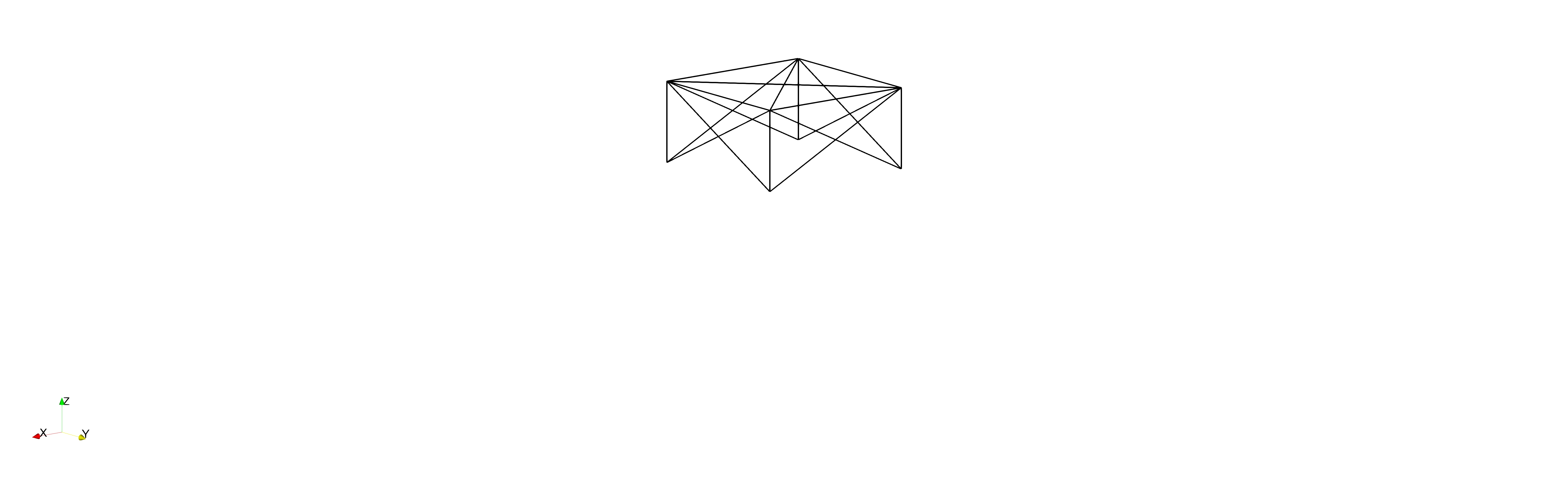
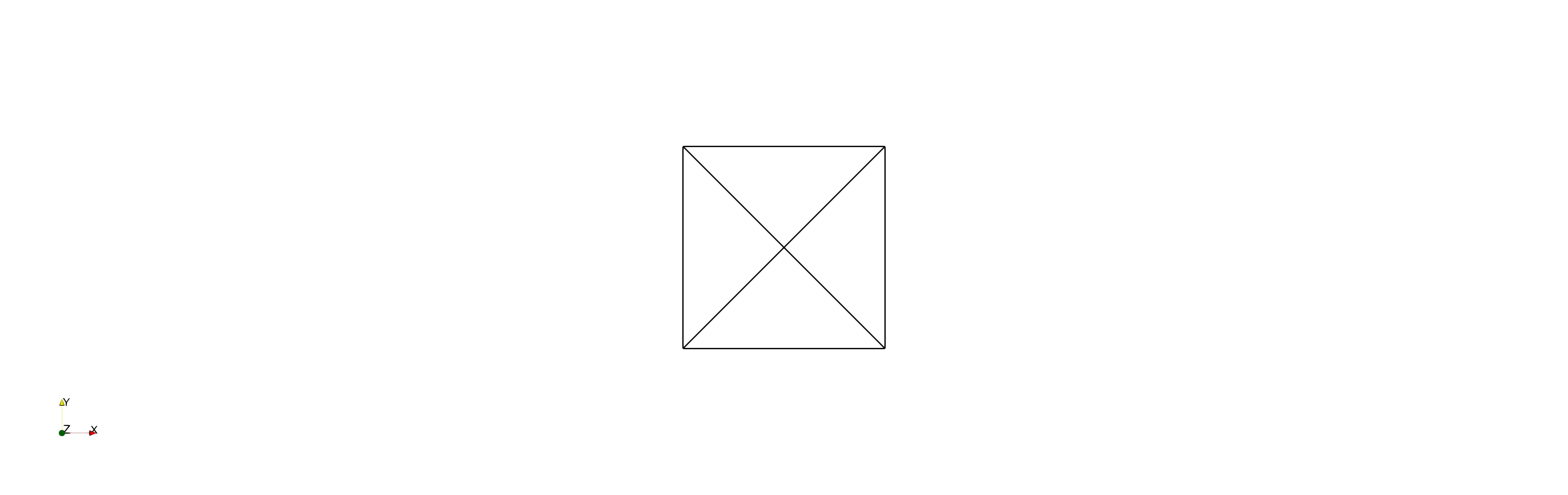
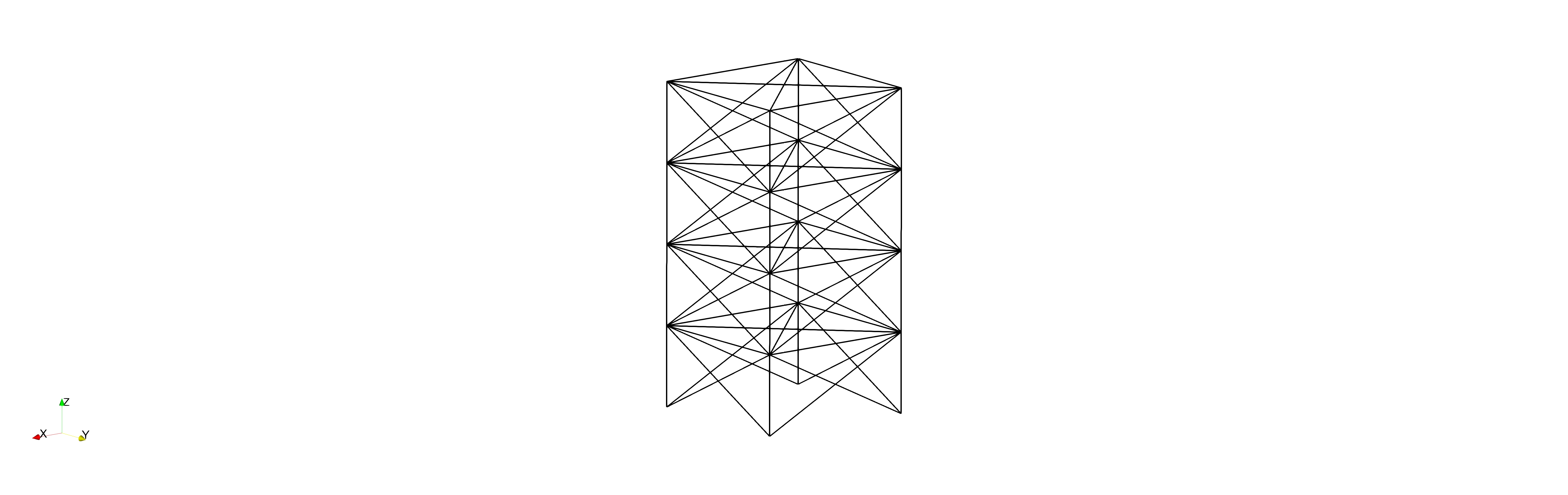
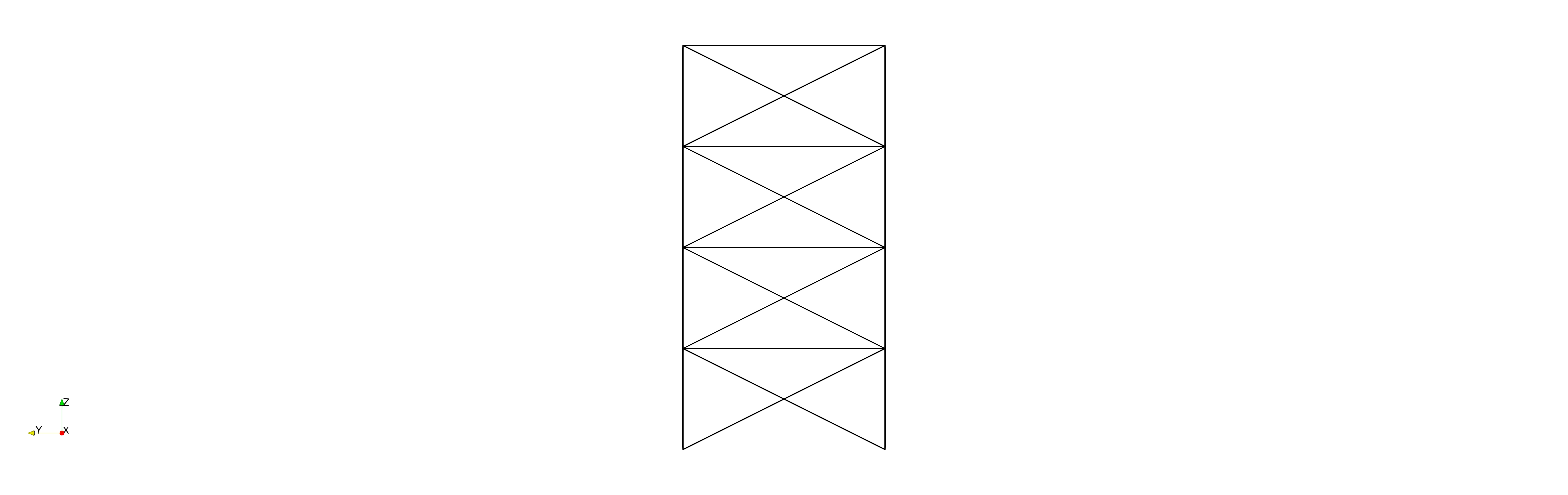
The 72-bar truss structure depicted in Figure 1 undergoes two load cases. In the first one, a force of f = [5000, 5000, 0]T lbf is applied to Node 1, and in the second load case, a force of f = [0, 0, −5000]T lbf is exerted on Nodes 1, 2, 3 and 4. The objective function for this problem is to minimize the structure’s mass and the design variables are the cross-sectional areas of all trusses (hence 72 variables in aggregate) selected from a discrete set given in Table 1. All members are made of an aluminum alloy with a density of 0.1lb/in3, Young’s modulus of 107 psi and yield stress of 25000 psi. For both load cases, the stress in all trusses must remain below the given yield stress and the displacement of Nodes 1, 2, 3 and 4 along X and Y axes must be bounded by ±0.25 in.

Figure 2 shows the convergence plot of the mean and standard deviation of the 10 GSMO and GA runs. Accordingly, the optimization routine advances smoothly and reaches convergence quite rapidly using both algorithms. Table 2 presents the optimum solution obtained by GSMO (the best one amongst the 10 runs), GA and those of other approaches reported in . For this problem, since the design variables are only categorical, in essence, there is no difference between GSMO and BiGSMO and the result of the latter is not provided.

As Can Be Seen, The Best Solution

generated by GSMO has a slight lead compared to those reported previously.

The Mean And

standard deviation of the 10 optimal results by GSMO are respectively 394.31 and 11.14, which may be taken as an affirmation of the fact that although a sampling process is involved in GSMO, the method consistently finds close optimum solutions (we have reviewed this claim in the subsequent case studies as well).

In this problem, perhaps the most significant advantage of GSMO is its computational time. Since GSMO is a gradient-based approach, it requires only one FE solve per Table 1: Categorical choices of the cross-sectional areas for the 72-bar truss structure

Areas (In2)

0.111, 0.141, 0.196, 0.250, 0.307, 0.391, 0.442, 0.563, 0.602, 0.766, 0.785, 0.994, 1.000, 1.228, 1.266, 1.457, 1.563, 1.620, 1.800, 1.990, 2.130, 2.380, 2.620, 2.630, 2.880, 2.930, 3.090, 3.130, 3.380, 3.470, 3.550, 3.630, 3.840, 3.870, 3.880, 4.180, 4.220, 4.490, 4.590, 4.800, 4.970, 5.120, 5.740, 7.220, 7.970, 8.530, 9.300, 10.85, 11.50, 13.50, 13.90, 14.20, 15.50, 16.00, 16.90, 18.80, 19.90, 22.00, 22.90, 24.50, 26.50, 28.00, 30.00, 33.50

14

optimization iteration leading to a total of 100 FE solves for each run. For this example, each GSMO run takes about 0.9 seconds on average on the computer specified earlier.

18

Figure 1: The 72-bar truss structure. The typical story is repeated 4 times along the Z axis. The node and element numbering also follows suit.

812-Bar Lattice Structure

In this example, the goal is to optimize the lattice structure shown in Figure 3 to have nonpositive Poisson’s ratios in X and Y directions. The lattice is symmetric with respect to XY, XZ and YZ planes and is composed of 4 by 4 unit cells depicted in Figure 3. It is pulled along the Z axis by 0.2 m, while the nodes on the outer edges of the mid-plane are expected to satisfy

(23)

where xf,i and x0,i are respectively final and initial x-coordinates, and yf,i and y0,i are respectively final and initial y-coordinates of Node i on the outer edges of the plane. Equation 23 means that the lattice structure must not shrink and possibly expand from the middle in both X and Y directions

15

Table 2: Categorical choices of the cross-sectional areas (in2) for the truss structure found by

388.01

while being pulled along the Z direction. Note that even though the deformations are large, we still model the structure assuming linear elasticity as the focus of this paper is optimization rather than simulation. In this example, the sole purpose is to satisfy the constraints expressed in (23), hence the constant function J = 0 is considered for the objective function. The lattice is discretized by Euler-Bernoulli beam elements all of which are made of a steel alloy with a Young’s modulus of 210 GPa and a Poisson’s ratio of 0.3.

This problem contains a mix of continuous and categorical design variables. The former variables include the orientation of all the 812 beams and the spatial position of the nodes interior to the structure (i.e., those not lying on the lattice’s top, bottom, front, back and side planes; 91 nodes in total). This leads to a total of 1085 continuous design variables. For the categorical variables, the 812 beams of the lattice are classified into 4 groups; those along the X, Y and Z axes as well as those along the unit cells’ diagonal directions. For each group, 4 cross-sectional choices exist. The

Related Journal Articles & DOI Links

Selected peer-reviewed publications relevant to 12 Lead ECG Acquisition. Click the DOI to access the full paper (may require institutional access).

Why Choose Us?

Bangalore guidance for robotics, Spectre and autonomous systems projects.