Uv Disinfection Monitoring

1

Optimized Coverage Planning for UV Surface Disinfection Jo˜ao Marcos Correia Marques1, Ramya Ramalingam2, Zherong Pan1 and Kris Hauser1 Abstract— UV radiation has been used as a disinfection strategy to deactivate a wide range of pathogens, but existing irradiation strategies do not ensure sufficient exposure of all environmental surfaces and/or require long disinfection times.

We present a near-optimal coverage planner for mobile UV dis- infection robots. The formulation optimizes the irradiation time efficiency, while ensuring that a sufficient dosage of radiation is received by each surface. The trajectory and dosage plan are optimized taking collision and light occlusion constraints into account. We propose a two-stage scheme to approximate the solution of the induced NP-hard optimization, and, for efficiency, perform key irradiance and occlusion calculations on a GPU. Empirical results show that our technique achieves more coverage for the same exposure time as strategies for existing UV robots, can be used to compare UV robot designs, and produces near-optimal plans. This is an extended version of the paper originally contributed to ICRA2021.

I. Introduction

The Covid-19 pandemic has encouraged worldwide inno- vation in methods for reducing the risk of disease trans- mission in hospitals, public transportation and other public spaces. One promising technology is ultraviolet (UV) disin- fection of surfaces, which has strong antimicrobial properties particularly in the UVC (200–280 nm) spectrum. UVC has long been known to deactivate a wide range of pathogens, such as Coronaviruses [1, 2], bacteria and protozoans .

Existing UV delivery approaches include air and water disinfection systems used in filtration and waste processing plants , as well as surface disinfection systems in the form of wands , overhead lights, pushcarts, and mobile robots

Carrying High-Power Uvc Lamps . Hospital Testing

has shown that a combination of standard manual cleaning followed by UVC surface irradiation has shown to be more effective in disinfecting environments than manual cleaning alone.

Dosing is an important factor in effective use of UVC, and is usually performed by following manufacturers’ guidelines. Although some UV disinfection robots also feature sensors that measure reflected radiant energy as an approximation of surface dosage, existing methods fail to disinfect certain parts of the environment . Two pitfalls are noted. The radiant fluence received by a surface is affected by the inverse square law, so fluence drops quickly as distance increases. Second, occlusions also affect the delivery of light into back-facing or *J. Marques and K. Hauser are partially supported by NSF Grant NRI-2025782. R. Ramalingam is supported by a CRA-WP DREU grant.

Usa

2R. Ramalingam is with the Dept. of Computer Science and the Dept. of Mathematics, Harvey Mudd College, Claremont, CA, USA

Fig. 1:

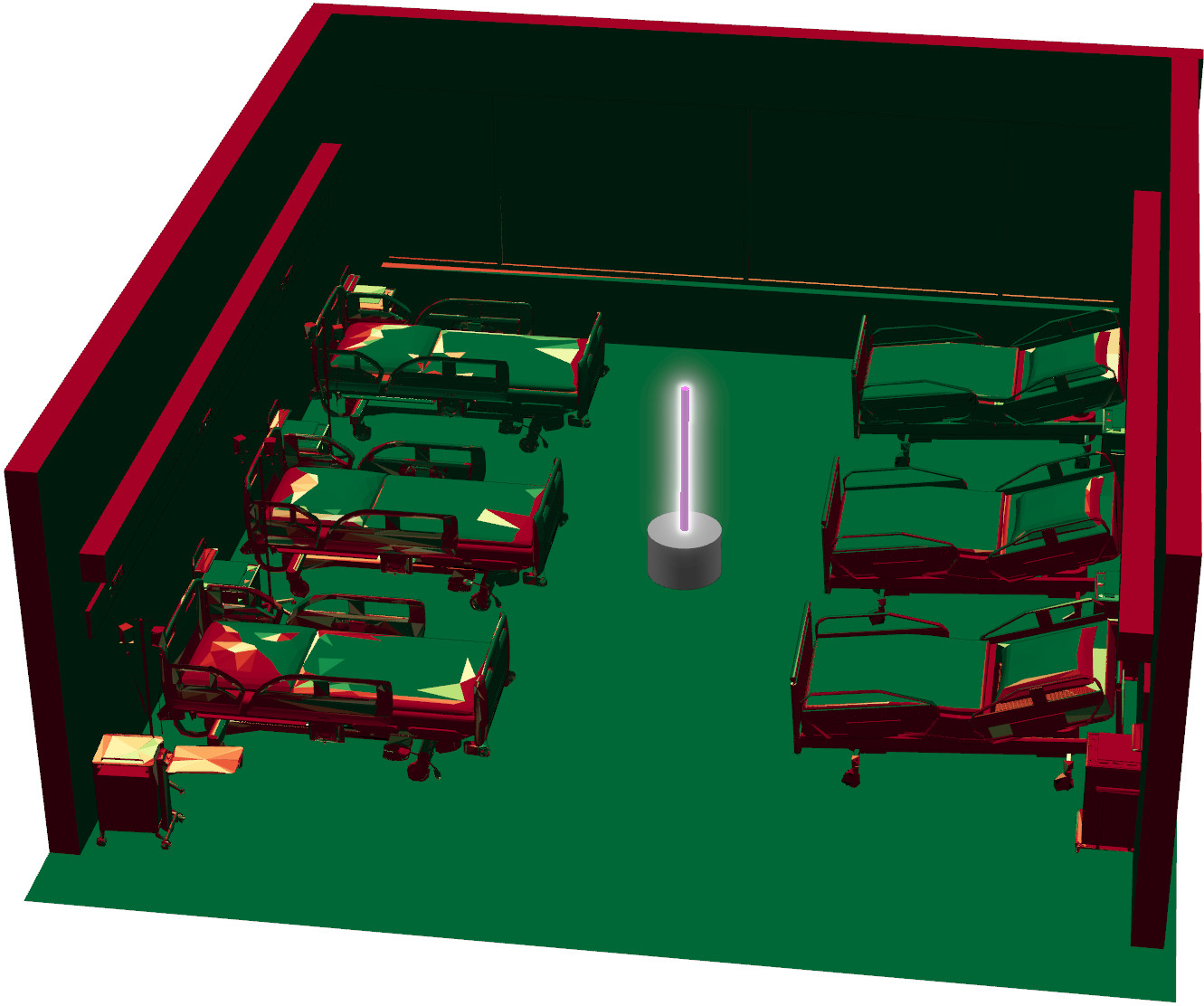
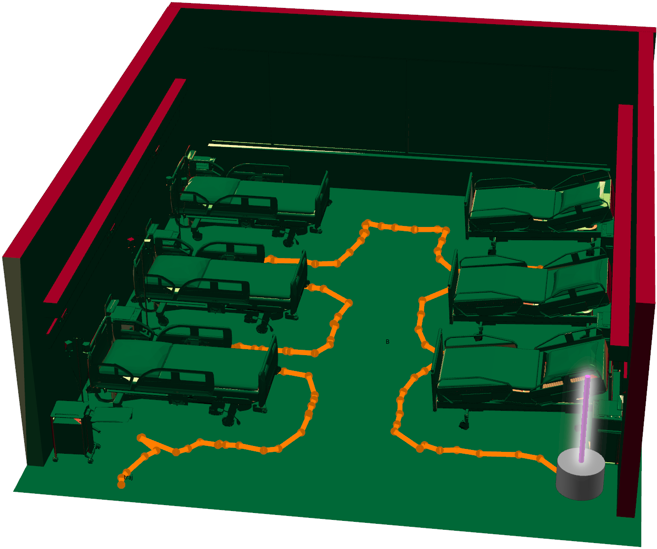
Comparison of a standard stationary mobile robot (top) against an optimized motion (bottom). Robot carries a tower light that emits UV radiation uniformly along its length. Surfaces are color coded by UV fluence received, with red indicating 0 J/m2 and green indicating 280 J/m2 or higher. A stationary light is unable to disinfect much of the environment after 30 minutes, while a mobile robot following our optimally computed trajectory (in orange) achieves almost complete coverage. (Best viewed in color) shadowed regions. These effects are illustrated in Figure 1, which shows a simulation of the irradiation of a hospital infirmary under a static UV tower, demonstrating ineffective disinfection of bedsides and occluded equipment.

We present a method for planning optimal trajectories of a mobile UV disinfection robot with dosing constraints. Our optimization can be configured to prioritize coverage of high- touch surfaces under a fixed time budget, or to guarantee the eventual full disinfection of all surfaces reachable by irradiation. The robot’s movement must be collision-free while conforming to the dosing constraints. We solve the problem by building a probabilistic roadmap in the robot’s configuration space, and then finding a tour of a subset

2

of configurations that optimizes the dose. The coverage problem on the roadmap can be cast as an NP-hard Mixed- Integer Linear Programming (MILP), but we propose an approximate two-stage solver that uses a Linear Program (LP) to find dwell times followed by a Traveling Salesman Problem (TSP) to find the tour. Experiments show that our solver is orders of magnitude faster than MILP with a loss of less than 3% of optimality. Moreover, dosage planning requires determination of an irradiance matrix that considers visibility and exposure of every surface patch from each candidate UV light pose, and we propose an approach that efficiently calculates this large matrix using a Graphics Processing Unit (GPU).

Ii. Related Work

Motion planning for UV disinfection bears a resemblance to two well-studied problems: coverage and inspection plan- ning. The goal of coverage planning [8, 9, 10, 11] is for every point in the freespace to be covered by the robot, while the goal of inspection planning [12, 13, 14, 15, 16] is for every point on an object surface to be visible from some point on the robot trajectory. The disinfection planning problem intro- duced in this paper adds an additional layer of complexity to inspection planning, where every point in an object surface must receive a certain amount of irradiance exposure. This scenario induces a joint problem of robot trajectory planning and disinfection time assignment. Compared with standard coverage and inspection planning, UV disinfection is applied routinely in healthcare facilities, public spaces, and food industries, and can take tens of minutes to ensure enough dosage. Therefore, achieving (near) optimality in reducing the disinfection time for a known environment, which is the focus of this paper, is more important than adapting to unknown environments or online re-planning as done in Refs. [13, 11].

Besides robotics, UV disinfection planning can be under- stood as an effort to model and control light transport. In this aspect, there is overlap with similar efforts in the field of radiation dosage planning [17, 18, 19, 20], rendering of Lambertian surfaces using boundary element method [21, 22, 23, 24] (otherwise known as radiosity), and optimization of light placements [25, 26]. The radiation dosage planning problem has the same goal as our problem, ensuring the delivery of sufficient amount of dosage to target volumes. An additional goal is to reduce the dosage as much as possible for the organs at risk. However, since geometric information of human organs is difficult to acquire, these methods are mostly heuristic and sub-optimal. Radiosity is used to only model light transportation, reflection, and absorption. Of particular interest is GPU-accelerated radiosity where the occlusion map is computed using GPU rasterization. A similar technique is used in this work, while indirect light reflections are ignored by our method as their contributions are assumed neglectable. Other works on lighting optimiza- tion for urban design or scientific data visualization [25, 26] also considers moving light sources, but these lights are fixed after the design phase.

Finally, Hu et al. present a pipeline for UV disin- fection of built environments, wherein 3D environments are reconstructed using off-the-shelf SLAM, while performing affordance estimation using a neural-network on the RGBD streams and projecting them into the generated map. The labels are then projected onto the 3D map and used to indicate areas that are likely to be contaminated and direct their robot to those segments, executing one of two disin- fection motion primitives on the environment - a scanning motion for flat segments and a circling motion for cylindrical shapes. They do not, however, provide any reasoning or experiments regarding the effectiveness of their disinfection strategy, focusing their results on the performance of the affordance estimates and on the mechanical feasibility of their disinfection primitives on a static robot. Their planning strategy also does not consider a disinfection tour, but limits itself to planning collision-free trajectories between the robot’s current position and a given area to be disinfected.

Iii. Uv Disinfection Trajectory Planning

Here we formalize the path planning problem for targeted UV disinfection first as a continuous, infinite-dimensional trajectory optimization problem, and then as a discrete ap- proximation.

A. Continuous Formulation

Let E ⊂R3 be the boundary of the environment, which is the surface to be disinfected. The disinfection is performed using a mobile robot equipped with a UV light, where C is the robot’s configuration space and Cfree is the freespace.

When the robot assumes any collision-free configuration x ∈ Cfree, each infinitesimal surface patch ds ∈E will receive a certain amount of radiative fluence per second. We model the radiative fluence distribution using a so-called Poynting vector function I(x,ds), such that the infinitesimal surface

(1)

where ds is the infinitesimal surface patch with outward normal n(s) and ⟨●,●⟩is the inner product. Note that I(x,ds) already encodes the effects of light mirror reflections and occlusions by the environment. For instance, in the case where there are full occlusions before reaching ds, this vector is zero. We denote τ(t) ∶R ↦Cfree as the trajectory in the robot configuration space parameterized in time t ∈[0,Tfinal]. The radiant fluence (also known as radiant exposure) of an infinitesimal surface patch ds from

0

Ids(τ(t))dt.

3

We define the minimum-time, continuous path planning

(3)

where f(τ, ˙τ,u) encodes the robot dynamics , u(t) is the control signal, umax is the control limits and µmin(ds) is the minimum disinfection fluence (dose) prescribed to the surface. The prescribed dose can be surface-dependent (e.g., to deliver more radiation to high-touch surfaces), but we set a constant µmin for notational simplicity. Eq. 3 is intractable due to the infinite number of constraints and the integral in Equation 2.

B. Discrete Formulation

Next, we formulate a discrete counterpart of (3). The surface E is discretized using a simplicial complex with N triangles, {si∣i = 1,⋯,N}. The robot can only take a discrete set of K configurations {x1,⋯,xK} ⊂Cfree.

Each configuration xk is called a vantage configuration. To simplify total irradiance calculations, we assume that the light source stops at each configuration xk in its trajectory for some dwelling time, denoted as tk ≥0, and emits no radiation during the transition between vantage configurations. Let t be the vector of K dwell times. We then discretize (1) and

K=1

Ii(xk)tk.

(5)

Suppose there exists a network of paths between configura- tions that satisfies kinematics and dynamics constraints. Let dkl ≥0 be the distance along the network between any xk and xl, with dkl = ∞if no path connects them. We then formulate the discrete version of (3) as a path subset selection problem.

We introduce binary variables zkl ∈{0,1}, each indicating whether the path dkl is used in the final path, and a vector z collecting each indicator. Then the discrete version of (3)

Z Connected

tk > 0 iff zkl = 1 or zlk = 1 for some l.

(6)

The last two conditions are consistency constraints, stating that the selected paths form a simply connected path, and the second ensures that the robot can only dwell on vantage configurations that are part of the selected path.

Iv. Proposed Solution

In this section, we propose a novel approximate algorithm to search for near-optimal coverage plans. The main steps of

Our Approach Are Listed Below:

1) Select vantage points {x1,⋯,xK′} and obtain the sub- set of vantage configurations {q1,⋯,qK} for feasible points (Detailed in Section IV-A).

2) Compute network R of paths between configurations using a PRM-style approach. Retain subset of reachable

3) Compute Irradiance Matrix Ii(Xk) (Sec.Iv-C)

4) Solve a LP for optimal dwell times t (Sec.IV-D) 5) Solve a TSP for a tour of all configurations qk for which

Dwell Time Is Nonzero, That Is Tk > 0 (Sec.Iv-D)

6) Execute the tour, stopping for time tk at each visited

Configuration Qk

We show in Appendix I, that Eq. (6) can be formulated as a Mixed Integer Linear Program (MILP). As vantage configurations grow increasingly dense and paths in the network R approach optimal paths, the MILP solution will approach the optimal solution to the original continuous problem (3). However, finding optimal MILP solutions is NP-hard - and finding suitable solutions usually gets harder with the amount of integer variables in the formulation of the problem - which in the case of the formulation in Appendix I scales with O(K2). We therefore opt to tackle this problem with a two-stage LP+TSP approach.

The LP first finds an dosage plan, in the form of dwell times to be spent at each vantage configuration, that is opti- mal assuming that the robot can instantly “teleport” between configurations. Second, the TSP finds the minimum-time traversal of the configurations with non-zero dwell times.

Assuming that the robot is sufficiently fast that irradiation is the limiting step, this strategy will produce near-optimal results.

Another issue to be addressed is that the integral in (4) does not have a closed form. We quickly compute an approx- imate irradiance vector from every vantage configuration and assemble them into an irradiance matrix using a GPU-based visibility check.

A. Vantage Configuration Selection

We first uniformly select a set of light positions in the task space, giving a superset {x1,⋯,xK′} of K′ light positions. For each light position, we solve the inverse kinematics problem for each robot IK(xk) = qk and insert qk into the vantage configuration set if a collision-free IK solution can be found. During IK feasibility computation, the robot’s geometry is dilated by 5 cm to discourage the use of “coiled“ configurations, since these induce harder planning problems.

The selection scheme of {x1,⋯,xK′} is robot-dependent. If the robot is able to move in 3-D, then they are drawn from an uniform grid in the bounding box of E in R3, but if the robot is constrained to 2D motion, like a mobile base, they are drawn from a gridding of the floorplan of E in R2.

B. Roadmap Computation

In this step we compute a PRM to attempt to connect the vantage configurations {q1,⋯,qK} with feasible paths. The PRM is an undirected graph R = (V,E) consisting of configurations q ∈Cfree, called “milestones“, and edges (a,b) ∈E between milestones a and b are straight line paths that are required to lie completely in the free space, that is, ab ∈Cfree. The feasibility of an edge is verified by linearly interpolating between configurations a and b and checking for collisions at regular intervals. In addition, we define the distance between two milestones a and b to be the length of the end-effector trajectory resulting from the linear interpolation between a and b in the workspace.

We then construct R with the following sampling scheme: 1) Add {q1,⋯,qK} as initial milestones of the PRM and try to connect pairs of nearby milestones if the edge between them is feasible.

2) Sample 4 thousand configurations at random from con- figuration space and attempt to connect them to the existing roadmap R. This random sampling is as fol- lows: 30% of the time, we sample uniformly at random

Of The Time, We Sample Within A Neighborhood Of A

target milestone, selected uniformly at random. If at the end of this step all target configurations lie in the same

Connected Component, Go To 6; Else, Go To 3

3) If the fraction of target milestones within the same connected component (φ) is smaller than 0.8, continue sampling milestones following the procedure in 2 in

Increments Of 200 Samples. Otherwise, Move To 4

4) If all target configurations are in the same connected component, go to 6; Else, if φ > 0.8, proceed with targeted sampling. Select one of the target milestones that is yet to be connected to the others uniformly at random, hereby named qfocus. Find the connected component to which qfocus belongs, Cfocus. Find the connected component containing the majority of the target milestones Cmajor.

5) Find the nearest neighbors between Cfocus and Cmajor, qfocusnear and qmajornear. Then, draw samples near either qfocusnear and qmajornear, uniformly at random.

After 10 samples have been drawn in this manner, return to 4. 6) Extract the configuration space trajectory between the target configurations from R, with no additional pro- cessing of the paths (i.e. shortcutting or a-posteriori trajectory optimization), and calculate the distances be- tween them.

Step 6 is introduced to help the planner focus its sampling on narrow passages in configuration space. After R is computed, vantage points that are not in the largest connected component are discarded. For the remain- ing points, the shortest paths in R between all pairs (qk,ql) are computed to form the distance matrix dkl. Note that one consequence of this targeted sampling approach is that milestones that lie in free space tend to be connected early on and, thus, tend to have more jagged paths between them.

Triangle Index

Fig. 2: Illustrating the GPU-based irradiance calculation. (a): The triangle index is rasterized into an environment map using geom- etry shader. (b): The power emission e(i, j) is precomputed. (c): The operation F[T[i, j]] += e(i, j) is performed using hardware

C. Discrete Radiative Fluence

We approximately calculate the radiative fluence matrix with entries Ii(xk). Note that a typical environment in 3D contains millions of triangles (N) and we will sample tens of thousands of potential vantage configurations (K).

Therefore, the matrix size Ii(xk) is huge and its calculation can typically become the bottleneck. We provide a GPU- based implementation that can calculate each column I∗(xk) in milliseconds.

The irradiance is a measure of the rate of radiant exposure, and is given in the units of watts per square meter. We first describe the simple case where the robot is a point light source, i.e. X = R3. We assume that reflected light is not a major source of illumination, so that the irradiance density received by the infinitesimal patch ds is given according to

(7)

where P is the power (or radiant flux) of the light source and s is the location of the infinitesimal surface patch. A patch is considered visible only if ⟨y −xk,n(s)⟩> 0 and no other surface lies closer to xk along the ray y −xk.

If no other triangles are in the way from xk to the entire triangle si, then the irradiance can be calculated according to , i.e. the integral of Equation 4 has closed form solution. However, when occlusion occurs, no closed form solution can be found for the per-triangle irradiance. Instead, our GPU-based implementation calculates the irradiance Ii(xk) by rasterization. This roughly follows the pipeline for radiosity calculations used in computer graphics [30, 23] disregarding Lambertian reflectance. Our implementation

(Fig. 2) Is Comprised Of The Following Steps:

●The scene is rasterized using a standard graphics pipeline, with the camera centered at xk. Each triangle’s index is rendered into the pixel buffer T bound to a cubemap texture (the visibility cube) using framebuffer object and a geometry shader . In the meantime, a Z-buffer is

5

used for visible surface determination. After rasterization, we store the value T[i,j] for each pixel (i,j) on the image plane. T[i,j] is the index of the closest triangle intersecting the ray from pixel (i,j) to xk. A void pixel indicates that no triangle is occupying the pixel.

●For each pixel T[i,j] containing a visible triangle, the amount of power e(i,j) emitted over the solid angle subtended by the pixel is calculated using and all power terms e(i,j) belonging to T[i,j] are summed up and stored in the triangle buffer F. This summation of e(i,j) is performed using the GPU’s hardware accelerated pixel-blending. In particular, we first set the triangle buffer F as the render target and store T[i,j] in the GPU buffer.

We then execute a shader program for each e(i,j), where we check T[i,j] for the index in F and use geometry shader to render a single pixel into F, with color equal to e(i,j) and pixel-blending turned on. The accumulated value for each triangle is the radiant flux, which measures irradiance integrated over the non-occluded area of the triangle.

●The radiant flux F[i] is divided by the area of each triangle to obtain the mean irradiance Ii(xk) = F[i]/∣si∣. Because this process will be performed repeatedly, the power emission e(i,j) for each pixel is precomputed and stored in a separate texture of the same dimensions as the rendered buffers, denoted as E, so that it can be retrieved with a single memory lookup. A note-worthy caveat of our method is the use of mean irradiance Ii(xk) = F[i]/∣si∣to replace the true uneven irradiance distribution within a single triangle, which can be remedied by having more finely discretized meshes.

Non-Point Light Sources: Our Procedure To Compute

Ii(xk) can be naturally extended to non-trivial light source shapes, such as an omnidirectional cylindrical light source. In those instances, the surface of light sources can be approx- imated by a set of evenly distributed point sources, where each point source emits an equal fraction of the light’s total radiant power. The total radiant flux is accumulated for each point before dividing by the area of each triangle to obtain the irradiance. More advanced shader programs such as can also be used to approximate the continuous integration of light contributions along the light source’s surface area on GPU. For light sources with uneven irradiance distribution, such as shielded or mirrored lights, we can replace the power emission texture E with a precomputed custom distribution.

If the light source is not standalone but mounted on a robot, then the position of the light source p is determined by its forward kinematics, which is denoted as p(xk) and plugged into Equation 7 in the place of xk, arriving at I(p(xk),n(s)).

D. Approximate Two-Stage Optimization

At this point, all related variables of Equation 6 have been calculated. The first stage proceeds by relaxing all zkl = 1 and derives an optimal set of dwell times. Assuming no transit time, the optimal dwell times can be determined by solving

(8)

A potential issue with Equation 8 is that it does not account for partially infeasible problems, which frequently occur in practice because some triangles sk are totally invisible from all vantage configurations. In these cases, Equation 8 will report infeasibility rather than return an approximate solution. To remedy this problem, we propose the following relaxed LP that always returns feasible solutions:

(9)

where pi denotes the infeasibility penalty of a triangle si and σi is a slack variable allowing all constraints to be satisfied in the worst case. We further constrain the time budget for disinfection to Tmax. With large penalties pi > ∥I∗(x∗)∥F and sufficiently large Tmax, the solution to the LP tends to set all σi = 0 and the solution to Equation 9 approaches the solution to Equation 8. When some surfaces are totally invisible or disinfection cannot be accomplished within the time budget, the LP solution accepts σi = µmin −µi > 0 for some indices i, thereby accepting penalty pi(µmin−µi). For prioritized surface patches si, a larger pi should be used so the LP tends to avoid positive σi. To solve Equation 9 we leverage the large-scale interior-point algorithm implemented in Gurobi .

The second stage in this approximate approach solves the TSP problem to find a tour amongst vantage points with nonzero dwell times, that is, minimizes transit times amongst edges {zkl∣tk > 0 ∧tl > 0}. While this problem is still NP- hard, it is solved over a much smaller set of candidate paths.

In addition, since it fits the traditional TSP formulation, we are able to leverage polynomial-time approximate TSP solvers, such as , which have near-optimal performance for relatively small euclidean TSP instances as the ones we encounter. Once the tour is found, the final disinfection tra- jectory is obtained by linearly interpolating in configuration space along the edges of the roadmap.

V. Experiments

Our experiments aim to answer the following questions: 1) How much better is the coverage of an optimally planned disinfection trajectory if compared to a single-

Point Strategy?

2) How large is the optimality penalty incurred by solving

Formulation?

3) How do different robot designs compare in terms of

(B) Our Method

Fig. 3: Empty room disinfected by the best stationary point (red dot) and by our method. Each surface is colored by its received fluence, and the optimized trajectory is drawn in red. (Best seen in

Color)

We use a simplified 2.5D experiment to test questions 1 and 2, and a realistic environment in 3D for question 3. In each experiment, all surfaces require a minimum dis- infection fluence µmin = 280 J/m2, which is a conservative estimate of the necessary fluence to induce a 3log10 reduc- tion in infectivity of SARS-Cov2 . In addition, the light is assumed to have a constant radiant flux, P, of 80 W and that the maximum speed of all robot end-effectors is 0.5 m/s.

A. Comparison With Static Illumination

First we evaluate disinfecting the walls of a 5m×5m empty room as a 2.5D problem. Walls are 2 m meters tall and a spherical point light source is used. We consider a discretized version of the room where each wall is subdivided into fixed-length subsegments, and irradiance from a point can be calculated analytically for rectangles . We consider a static illumination strategy that places the disinfection light to have maximum coverage over the obstacle space, allowing it to irradiate the surfaces for as long as necessary to fully disinfect its visible surfaces. In our method, we treat the robot as a cylindrical base of radius 10 cm, and constrain the movement of the light to a plane at height 1 m. Vantage points are sampled along a 0.1 m grid. The static method takes 143.7 minutes to reach full room disinfection, while ours does so in 95.6 minutes, including movement time between vantage points - the contrast between solutions is

Illustrated In Figure 3

Next, we randomly generate 25 2.5D rooms in a 4 m×4 m area and with 2 m tall polygonal obstacles. Each world contains a random number of obstacles (between 7 and 19), with each obstacle randomly generated by scaling, shearing and displacing regular polygons. Visibilities of each segment from a given vantage point are determined by creating a visibility graph amongst vantage points and segment midpoints . Figure 4 shows the output for one example. Note that for our method, all segments are covered, and few segments are overexposed. Figure 5 shows results averaged over all rooms, indicating that our proposed method consistently disinfects 100% of the environment, whereas the optimal static illumination only disinfects 35%. Moreover, to disinfect the visible segments, static illumination requires approximately 2 orders of magnitude more time.

(B) Our Method

Fig. 4: Same room disinfected by the best stationary point (red dot) and by our method. Each surface is colored by its received fluence and the trajectory is drawn in red. (Best seen in color)

Single Point

Fig. 5: 2.5D Disinfection performance comparisons with best single

B. Comparison Against Milp Formulation

Next, we compare the two-stage scheme and the glob- ally optimal MILP formulation described in our extended report . We limited the point robot to travel along a grid with 0.5m spacing, resulting in ≈64 candidate vantage points and ≈4k boolean variables in the MILP(to ensure MILP feasibility within constrained time). These results are illus- trated in Figure 6. Columns 1, 2 indicate the mean percentage difference between MILP and LP solutions; columns 3 and 4 indicate the mean percentage of dwell time w.r.t. the total disinfection time in each solution and column 5 is the mean value of the ratio between the computation time of the MILP over the computation time for the LP+TSP. Note that path lengths differ, on average, less than 10% between the two solution methods - which is evidenced by the mean difference of less than 5% in total disinfection time. In addition, we verify our initial assumption that dwell times make up the majority of disinfection time, since they represent over 90% of the total disinfection times in both cases. Moreover, the two-stage approach is 6 times faster, on average, to compute than the optimal MILP solution - even in examples with coarse grid. Note that in a grid with twice the resolution (≈ 256 candidate vantage points - ≈65k boolean variables in the MILP), we could not get solutions within 2 hours for the MILP formulation, while the LP+TSP solutions took about 5 seconds to compute, on average. Additional experiments evaluating the impact of grid resolution and environment discretization resolution can be found in Appendix II.

Related Journal Articles & DOI Links

Selected peer-reviewed publications relevant to 12 Lead ECG Acquisition. Click the DOI to access the full paper (may require institutional access).

Why Choose Us?

Bangalore guidance for robotics, Spectre and autonomous systems projects.