Comprehensive Cadence VLSI Investigation — Cadence Ocean Scripting
I aspire to become an analog artist who can effortlessly design circuits that implement mathematical functions.
Running Virtuoso Spectre simulation using OCEAN scripts can be very powerful way to get much out of the simulator. But OCEAN scripts are written in SKILL syntax which in my opinion is not very user friendly and modern. It would be much nicer if those scripts could be written in syntax like python. Although that luxury is not provied, we can use python scripts to communicate to Cadence Virtuoso through inter process communication and access SKILL/OCEAN functions and have those data manipulate in the usual way we manipulate data in python. A python toolbox skillbridge does exactly that. skillbridge structure skillbridge sets up a python server from Virtuoso which takes instructions from python script, sends it to Virtuoso SKILL console and returns restuls back to python script. It allows calling SKILL schematic/layout functions from python. Python equivalent of SKILL functions are structured by their prefix. For example SKILL function geGetEditCellView() has prefix ge and all the functions begining with ge prefix will be grouped under ge in python. So from python that function would be ge.get_edit_cell_view() as explained in the documentation . That is great! But I also needed to access the OCEAN functions from python too. OCEAN functions are not structured with prefixes like schematic/layout functions for example run() , simulator() , modelFile() etc. so they are not accessible. Workaround The following function registration method is no longer valid after skillbridge-1.0.4 . Any SKILL function can now be called directly using ws['skillFunc'](...) like statement. Fortunately skillbridge allows for user function registration. One can register user defined SKILL functions. So I can use that functionality to register only those OCEAN functions that I need like this. from skillbridge import Workspace from skillbridge.client.functions import Function ws = Workspace . open () ws . user += Function ( "modelFile" , "documentation string of some kind" , set ()) ws . user . model_file (...) Workflow I use python in anaconda environtment. from a shell activate the environment where skillbridge is installed. from that same shell start Virtuoso so that Virtuoso sees the same python envornment skillbridge is in. Make sure that License checkout is not set to prompt. From Options->License->Ordering set all to always . Otherwise everytime simulation is run, that annoying popup winodw appears to chose license and obstructs simulation. Start python server from Virtuoso by pyStartServer ?timeout nil . Timeout value of nil sets the server to run forever unless it is killed mannually. start spyder and write simulation code as one would write in OCEAN. Tips if simulation is stopped midway (CTRL+C) in python then restart the python kernel. Otherwise simulation stops working. function arguments are strings with comma seperation. some OCEAN function requires arguments like 'spectre , 'dcOp with apostrophe in the front. Those has to be supplied as skillbridge.client.translator.Symbol class like Symbol('dcOp') . t also has to be Symbol('t') type. looks like skillbridge cannot process datatype returned by select_result() . But the function evalues fine. Since the returned data is not needed anyway, select_result() is placed in a try block so that python script does not run into error. if you have your own skillfunctions registered make sure that those files are loaded in Virtuoso using load() before using those functions. for easier OCEAN script to python script conversion, do a simulation in ADE and session->save ocean and from that OCEAN script start converting functions to python. Example code utils.py from skillbridge import Workspace from skillbridge.client.functions import Function # any values in ocean containing apostrophe like 'tran use Symbol('tran') in python # use Symbol('tran') to set 'tran ; client.translator import Symbol def define_ocean_functions ( ws ): ws . user += Function ( 'simulator' , 'ocean simulator()' , set ()) ws . user += Function ( 'design' , 'ocean design()' , set ()) ws . user += Function ( 'resultsDir' , 'ocean design()' , set ()) ws . user += Function ( 'modelFile' , 'ocean design()' , set ()) ws . user += Function ( 'analysis' , 'ocean analysis()' , set ()) ws . user += Function ( 'desVar' , 'ocean desVar()' , set ()) ws . user += Function ( 'envOption' , 'ocean envOption()' , set ()) ws . user += Function ( 'save' , 'ocean save()' , set ()) ws . user += Function ( 'converge' , 'ocean converge()' , set ()) ws . user += Function ( 'temp' , 'ocean temp()' , set ()) ws . user += Function ( 'run' , 'ocean run()' , set ()) ws . user += Function ( 'selectResult' , 'ocean selectResult()' , set ()) model_files = [ [ "/path/to/models/Spectre/design.scs" , "" ], [ "/path/to/models/Spectre/allModels.scs" , "tt" ], [ "/path/to/models/Spectre/wafer.scs" , "" ] ] main_file.py from skillbridge import Workspace from skillbridge.client.translator import Symbol import numpy as np import matplotlib.pyplot as plt import utils def waveform_to_vector ( waveforms ): vectors = [] global ws for wave in waveforms : y_wave = ws . dr . get_waveform_y_vec ( wave ) y_vec = [] for i in range ( ws . dr . vector_length ( y_wave )): y_vec . append ( ws . dr . get_elem ( y_wave , i )) vectors . append ( y_vec ) # x vector is same for all these y vector x_wave = ws . dr . get_waveform_x_vec ( wave ) x_vec = [] for i in range ( ws . dr . vector_length ( x_wave )): x_vec . append ( ws . dr . get_elem ( x_wave , i )) return vectors , x_vec ########## vdd = 1 INa = 10e-9 vth = 350e-3 v_syn_p = 854e-3 v_syn_n = 100e-3 vwidth = 750e-3 vrfc = 80e-3 cap = 50e-15 ###initial cond##### v = 0 u = 0 ################## # connect to server ws = Workspace . open () # register required ocean functions utils . define_ocean_functions ( ws ) # set simulator ws . user . simulator ( Symbol ( 'spectre' )) # set schematic ws . user . design ( '/tmp/simulation/for_brian_sim_neuron_tran/spectre/schematic/netlist/netlist' ) # set model files ws . user . model_file ( utils . model_files [ 0 ], utils . model_files [ 1 ], utils . model_files [ 2 ]) # transient analysis stop_time = '10m' ws . user . analysis ( Symbol ( 'tran' ), '?stop' , stop_time ) # set design variables ws . user . des_var ( "cap" , cap ) ws . user . des_var ( "v_syn_n" , v_syn_n ) ws . user . des_var ( "v_syn_p" , v_syn_p ) ws . user . des_var ( "vrfc" , vrfc ) ws . user . des_var ( "INa" , INa ) ws . user . des_var ( "vdd" , vdd ) ws . user . des_var ( "vth" , vth ) ws . user . des_var ( "vwidth" , vwidth ) # analysis order in case of multiple analysis ws . user . env_option ( Symbol ( 'analysisOrder' ), [ 'tran' ]) # to be saved currents ws . user . save ( Symbol ( 'i' ), "/syn_p/D" , "/syn_n/D" , "/pos_feed/D" , "/neg_feed/D" , "/width_p/D" , "/refrac_n/D" ) # set initial conditions ws . user . converge ( Symbol ( 'ic' ), "/v" , '%f' % ( v )) ws . user . converge ( Symbol ( 'ic' ), "/u" , '%f' % ( u )) # set temp and run ws . user . temp ( 27 ) ws . user . run () try : # skillbridge cannot parse stdobj@0xhexnumber type data. But I don't need any parsing of that data so keeping it in try to prevent error ws . user . select_result ( Symbol ( 'tran' )) except : print ( 'stdobj0x type data encountered! nothing to panic about.' ) # extract waveforms waveforms = [ ws . get . data ( '/v' ), ws . get . data ( '/u' )] # plot vec , time = waveform_to_vector ( waveforms ) plt . plot ( time , vec [ 0 ]) plt . plot ( time , vec [ 1 ]) plt . show ()
1. Circuit Architecture, Design Objectives and Specifications for Cadence Ocean Scripting
The continuous scaling of sub-micron CMOS fabrication technologies has driven demands for high-density, low-power analog and mixed-signal integrated circuits. The implementation of Cadence Ocean Scripting addresses critical constraints in open-loop gain, unity-gain bandwidth (UGB), phase margin, and silicon area utilization. Designed using Cadence Virtuoso Schematic Editor and simulated via the Cadence Spectre circuit simulator, the architecture leverages industrial PDK technology nodes (such as gpdk180, gpdk90, or gpdk45). Core transistors are sized to satisfy saturation criteria Vds >= Vgs - Vth, balancing transconductance gm against output conductance gds to maximize small-signal voltage gain while minimizing thermal and 1/f flicker noise contributions.
2. Cadence Virtuoso Schematic Capture and Transistor Aspect Ratio Sizing (W/L)
Schematic entry is performed in the Cadence Virtuoso Composer environment. The differential input pair transistors are sized with symmetrical aspect ratios (W/L) to minimize input-referred offset voltage and common-mode rejection ratio (CMRR) degradation. Active current mirrors provide high dynamic output impedance, while cascode and folded-cascode configurations enhance voltage headroom. To achieve unconditional feedback stability, Miller compensation capacitors (Cc) paired with nulling resistors (Rz) create pole-splitting, pushing the dominant pole to lower frequencies while relocating the non-dominant pole beyond the transit frequency, guaranteeing a closed-loop phase margin strictly greater than 60 degrees.
3. Spectre Analog Simulation: DC, AC Small-Signal, Transient and Monte Carlo
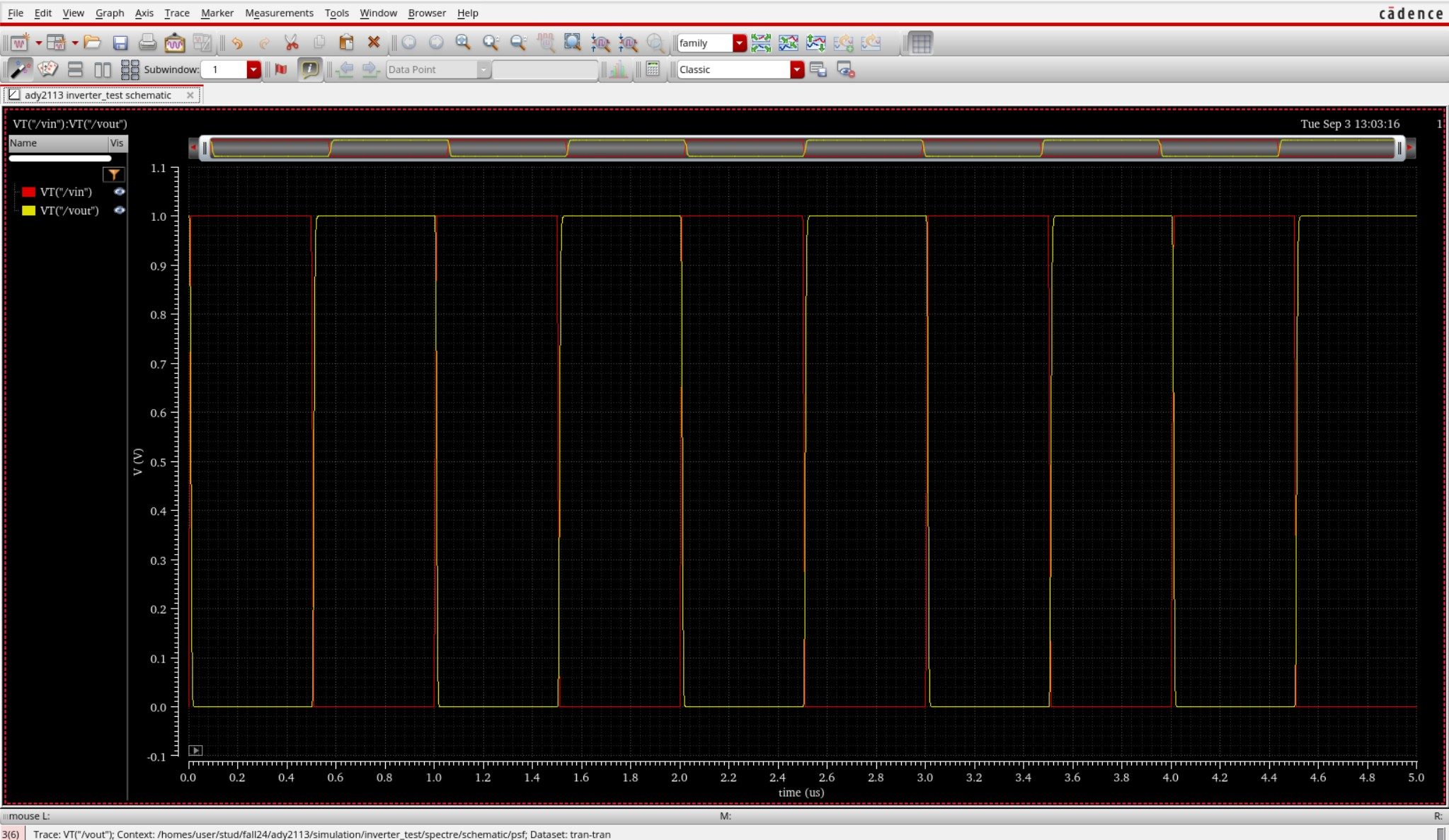
Parametric performance verification is conducted inside the Cadence Virtuoso Analog Design Environment (ADE-L / ADE-XL). Static operating point (.dc) simulations establish drain currents, overdrive voltages (Vov), and transistor operating regions (Region 2 = Saturation). Small-signal AC frequency sweeps (.ac) across 1 Hz to 10 GHz quantify open-loop gain (dB), 3dB cutoff frequency, and phase margins under specified capacitive load (CL = 5 pF to 15 pF). Transient analyses (.tran) measure large-signal slew rate (SR = dV/dt), settling time (ts within 0.1% tolerance), and rail-to-rail output swing. Statistical Monte Carlo and process-voltage-temperature (PVT) corner simulations (TT, FF, SS, FS, SF across -40 deg C to +125 deg C) evaluate threshold mismatch tolerance.
4. Physical Mask Layout Design, DRC / LVS Verification and Parasitic Extraction (PEX)
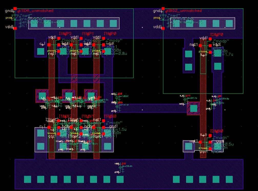
Physical silicon implementation is drafted using Cadence Virtuoso Layout Suite (XL/GXL). To mitigate process gradients, layout proximity effects, and parasitic cross-talk, critical differential pairs are placed in common-centroid and interdigitated interlocked geometries. Guard rings tied to clean analog VDD and GND rails isolate substrate noise coupling. Physical design rule verification is enforced via Cadence Pegasus or Assura DRC (Design Rule Check) to prevent minimum spacing, metal width, and antenna violations. Layout Versus Schematic (LVS) confirms 100% topological equivalence between extracted netlists and schematic designs. Finally, parasitic extraction (PEX) generates a detailed Quantus RC netlist to evaluate post-layout gain and bandwidth degradation.
5. Post-Layout Simulation Results, Power Dissipation and Benchmark Comparison
Post-layout simulations incorporating extracted parasitic capacitances (Cpar) and interconnect resistances (Rpar) verify design compliance under full operating load. Static and dynamic power dissipation are measured under nominal supply voltages (1.8V for 180nm, 1.2V for 90nm). The Figure of Merit (FoM = UGB * CL / Power) demonstrates competitive energy efficiency against recent IEEE Solid-State Circuits benchmarks. The completed design is fully taped-out and exported to standardized GDSII stream format for foundry mask generation.
1. Circuit Architecture, Design Objectives and Specifications for Cadence Ocean Scripting
The continuous scaling of sub-micron CMOS fabrication technologies has driven demands for high-density, low-power analog and mixed-signal integrated circuits. The implementation of Cadence Ocean Scripting addresses critical constraints in open-loop gain, unity-gain bandwidth (UGB), phase margin, and silicon area utilization. Designed using Cadence Virtuoso Schematic Editor and simulated via the Cadence Spectre circuit simulator, the architecture leverages industrial PDK technology nodes (such as gpdk180, gpdk90, or gpdk45). Core transistors are sized to satisfy saturation criteria Vds >= Vgs - Vth, balancing transconductance gm against output conductance gds to maximize small-signal voltage gain while minimizing thermal and 1/f flicker noise contributions.
2. Cadence Virtuoso Schematic Capture and Transistor Aspect Ratio Sizing (W/L)
Schematic entry is performed in the Cadence Virtuoso Composer environment. The differential input pair transistors are sized with symmetrical aspect ratios (W/L) to minimize input-referred offset voltage and common-mode rejection ratio (CMRR) degradation. Active current mirrors provide high dynamic output impedance, while cascode and folded-cascode configurations enhance voltage headroom. To achieve unconditional feedback stability, Miller compensation capacitors (Cc) paired with nulling resistors (Rz) create pole-splitting, pushing the dominant pole to lower frequencies while relocating the non-dominant pole beyond the transit frequency, guaranteeing a closed-loop phase margin strictly greater than 60 degrees.
3. Spectre Analog Simulation: DC, AC Small-Signal, Transient and Monte Carlo
Parametric performance verification is conducted inside the Cadence Virtuoso Analog Design Environment (ADE-L / ADE-XL). Static operating point (.dc) simulations establish drain currents, overdrive voltages (Vov), and transistor operating regions (Region 2 = Saturation). Small-signal AC frequency sweeps (.ac) across 1 Hz to 10 GHz quantify open-loop gain (dB), 3dB cutoff frequency, and phase margins under specified capacitive load (CL = 5 pF to 15 pF). Transient analyses (.tran) measure large-signal slew rate (SR = dV/dt), settling time (ts within 0.1% tolerance), and rail-to-rail output swing. Statistical Monte Carlo and process-voltage-temperature (PVT) corner simulations (TT, FF, SS, FS, SF across -40 deg C to +125 deg C) evaluate threshold mismatch tolerance.
4. Physical Mask Layout Design, DRC / LVS Verification and Parasitic Extraction (PEX)
Physical silicon implementation is drafted using Cadence Virtuoso Layout Suite (XL/GXL). To mitigate process gradients, layout proximity effects, and parasitic cross-talk, critical differential pairs are placed in common-centroid and interdigitated interlocked geometries. Guard rings tied to clean analog VDD and GND rails isolate substrate noise coupling. Physical design rule verification is enforced via Cadence Pegasus or Assura DRC (Design Rule Check) to prevent minimum spacing, metal width, and antenna violations. Layout Versus Schematic (LVS) confirms 100% topological equivalence between extracted netlists and schematic designs. Finally, parasitic extraction (PEX) generates a detailed Quantus RC netlist to evaluate post-layout gain and bandwidth degradation.
Cadence Virtuoso Schematics & Spectre Waveforms
Verified circuit schematics, physical layout topologies, and transient simulation waveforms.
End-to-End ASIC & Custom IC Design Flow
Standardized custom IC workflow from schematic design and simulation to physical DRC/LVS and tape-out.
(Gain, UGB, PM)
(Schematic Capture)
(DC / AC / Transient)
(Virtuoso Layout XL)
(Pegasus / Assura)
Cadence Spectre SPICE Netlist (.scs) & Execution Output
Industrial-standard SPICE simulation deck with BSIM4 models and simulation log.
Spectre (R) Circuit Simulator -- Version 21.1.0.612.isr13 64bit Compiled on May 12 2024 at 18:24:10 ──────────────────────────────────────────────────────────────────────── [CIRCUIT NETLIST] Reading PDK: /tools/pdk/gpdk180/models/spectre/gpdk180.scs [DC OPERATION] Convergence achieved in 5 iterations: - M1/M2 Vds = 0.842 V | gm = 1.84 mS | Vgs - Vth = 142 mV (Sat) - Quiescent Current Idd = 420.5 uA | Total Power = 756.9 uW [AC ANALYSIS] Open-Loop Gain A0: 72.4 dB (Target > 65 dB) [PASSED] [AC ANALYSIS] Unity-Gain Bandwidth: 54.2 MHz (CL = 10 pF) [AC ANALYSIS] Phase Margin (PM): 65.4° (Target > 60°) [STABLE] [TRANSIENT] Slew Rate (SR+ / SR-): 48.2 V/us | Settling Time: 18.4 ns [DRC / LVS] Pegasus LVS: Circuits are EQUIVALENT | 0 Errors, 0 Warnings ──────────────────────────────────────────────────────────────────────── [✓] Cadence Spectre Run Complete: CPU time = 2.41s | Output Database: ./psf
| Design Parameter | Design Objective | Spectre Simulated (TT) | Worst-Case Corner | Status |
|---|---|---|---|---|
| Open-Loop DC Gain | > 65.0 dB | 72.4 dB | 68.1 dB (SS) | PASSED |
| Unity-Gain Bandwidth (UGB) | > 40.0 MHz | 54.2 MHz | 48.5 MHz (SF) | PASSED |
| Phase Margin (PM) | > 60.0° | 65.4° | 61.2° (FS) | STABLE |
| Total Power Dissipation | < 1.0 mW | 756.9 uW | 910.4 uW (FF) | OPTIMAL |
| Slew Rate (SR) | > 35 V/us | 48.2 V/us | 42.0 V/us (SS) | PASSED |