Comprehensive Cadence VLSI Investigation — Floorplanning In Cadence Innovus
🏗️ Floorplanning in Cadence Innovus 📖 What is Floorplanning? Floorplanning is the first major stage of the ASIC Physical Design Flow , where the physical structure of the integrated circuit (IC) is established. It defines the die area , core dimensions , placement region , power distribution network (PDN) , and routing resources , creating the foundation for placement, clock tree synthesis, and routing. A well-planned floorplan minimizes routing congestion, improves timing performance, optimizes power distribution, and enhances the overall quality of the final layout. 📋 Requirements Before Floorplanning Before starting floorplanning in Cadence Innovus , the following design inputs are required. 1️⃣ Technology Files Technology LEF (.lef) – Defines routing layers, via rules, manufacturing grid, and technology information. Macro LEF (.lef) – Describes the physical dimensions and pin locations of standard cells and macros. Liberty File (.lib) – Contains timing, power, and functional characteristics of the standard cell library. 2️⃣ Logical Design Inputs Synthesized Gate-Level Netlist (.v) generated from Cadence Genus . SDC Constraint File (.sdc) containing: Clock Definitions Input Delays Output Delays Timing Constraints 3️⃣ Physical Design Parameters Core Utilization Aspect Ratio Core Margins Placement Site Information Routing Layer Preferences 4️⃣ Power Planning Requirements Power Net ( VDD ) Ground Net ( VSS ) Power Rings Power Stripes Follow Pins 🧩 Floorplanning Flow 1️⃣ Import Design Load all required design files into Cadence Innovus . Input Files ✔️ Synthesized Netlist ✔️ Technology LEF ✔️ Macro LEF ✔️ Liberty Library ✔️ SDC Constraints 2️⃣ Initialize Floorplan Define the physical dimensions of the design. Typical parameters include: Core Utilization Aspect Ratio Core Offset Placement Site The objective is to allocate sufficient routing space while maximizing silicon utilization. 3️⃣ Power Planning Create the Power Distribution Network (PDN) . This stage includes: Power Rings Horizontal Power Stripes Vertical Power Stripes The PDN ensures reliable power delivery across the entire design while minimizing IR drop and voltage fluctuations. 4️⃣ Special Routing (SRoute) Special Routing establishes dedicated power connectivity by connecting: Standard Cell Power Pins Power Rings Power Stripes Core Power Nets (VDD/VSS) This step prepares the design for placement and signal routing. 5️⃣ Floorplan Verification Verify the following before proceeding: ✔️ Core Boundary ✔️ Placement Rows ✔️ Power Ring Connectivity ✔️ Power Stripe Connectivity ✔️ Available Routing Resources Any floorplanning issues should be resolved before the placement stage. 🎯 Objectives of Floorplanning Optimize chip area utilization Minimize routing congestion Improve timing performance Enable efficient power delivery Reduce overall wirelength Prepare the design for placement and clock tree synthesis 📦 Deliverables The floorplanning stage generates: Initialized Core Layout Placement Rows Power Rings Power Stripes Floorplan Database The quality of the floorplan significantly influences the final performance, power, area, and manufacturability of the ASIC design.
Floorplanning is the first major stage of the ASIC Physical Design Flow , where the physical structure of the integrated circuit (IC) is established. It defines the die area , core dimensions , placement region , power distribution network (PDN) , and routing resources , creating the foundation for placement, clock tree synthesis, and routing.
A well-planned floorplan minimizes routing congestion, improves timing performance, optimizes power distribution, and enhances the overall quality of the final layout.
Before starting floorplanning in Cadence Innovus , the following design inputs are required.
The objective is to allocate sufficient routing space while maximizing silicon utilization.
The PDN ensures reliable power delivery across the entire design while minimizing IR drop and voltage fluctuations.
The quality of the floorplan significantly influences the final performance, power, area, and manufacturability of the ASIC design.
GDS Layout Engineer A layout engineer's day starts with opening a GDS file Parse · Statistics · Visualize · Compare · Merge · Verify 🎯 What is this? What does a layout engineer's daily work look like? "How many layers are in this GDS?" → See at a glance "What changed from the last revision?" → Auto-compare, layer area changes "How do I stitch these sub-modules together?" → Merge with one command "How large is this module?" → Layer-by-layer statistics, precise to each layer "Boss wants to see what the layout looks like" → Export SVG, open in browser This skill automates all these repetitive tasks, so you can focus on what really needs thinking. ✨ Core Capabilities ┌─────────────────────────────────────────────────────────────┐ │ chip_top.gds │ │ │ │ ├── 📋 gds_info.py → Cell tree, layer list, bbox │ │ ├── 📊 gds_layer_stats → Layer count/area/density, CSV │ │ ├── 🎨 gds_to_svg.py → SVG visualization, layer filter │ │ ├── ⚖️ gds_compare.py → Compare two versions, find changes│ │ ├── 🔗 gds_merge.py → Merge multiple files, auto-offset│ │ └── 📐 cdl_to_xschem.py → CDL netlist to xschem schematic │ │ │ │ references/ → GDS format spec, layer mapping, DRC rules │ │ assets/ → Sky130 DRC template, layer map CSV template │ └─────────────────────────────────────────────────────────────┘ 🚀 Quick Start Install Dependencies pip install gdspy # Required: GDSII file I/O pip install svgwrite # Optional: SVG visualization 30-Second Experience # 1. See what's in this GDS python scripts/gds_info.py chip_top.gds # 2. Layer area statistics python scripts/gds_layer_stats.py chip_top.gds # 3. Export SVG preview python scripts/gds_to_svg.py chip_top.gds -o preview.svg # Open preview.svg in your browser # 4. Compare two versions python scripts/gds_compare.py old.gds new.gds # 5. Merge multiple modules python scripts/gds_merge.py analog.gds digital.gds -o chip.gds 📖 Typical Use Cases Case 1: First Time with an Unfamiliar GDS # Check basic information first python scripts/gds_info.py mystery.gds Output: ================================================== File: mystery.gds Top Cell: TOP Total Cells: 127 --- Cell Tree --- TOP ├─ ANALOG_BLOCK │ ├─ OTA_CORE │ └─ BIAS_GEN ├─ DIGITAL_BLOCK │ ├─ COUNTER [×8] │ └─ FSM └─ PAD_FRAME --- Layer List (23 unique pairs) --- (1, 0) ← Well (2, 0) ← Active (30, 0) ← Poly (44, 0) ← Metal1 ... --- Bounding Box --- X: 0.000 ~ 2400.000 (width=2400.000 um) Y: 0.000 ~ 1800.000 (height=1800.000 um) ================================================== Instantly see this is a mixed-signal chip (analog + digital), 127 cells, layer definitions look normal. Case 2: Check Metal Density Must verify metal density before tape-out, otherwise CMP will cause issues: python scripts/gds_layer_stats.py chip.gds --csv density.csv Output: ====================================================================== File: chip.gds | Cell: TOP | Layout Area: 4320000.00 um² ====================================================================== Layer/Dtype Count Area (um²) Density ---------------------------------------------------------------------- ( 44, 0) 45230 864000.00 20.00% ← Metal1 ( 45, 0) 32100 691200.00 16.00% ← Metal2 ... TOTAL 182000 1728000.00 40.00% ====================================================================== Instantly see Metal1/Metal2 density is low, need to add dummy fill. Case 3: Revision Comparison Made a revision, want to confirm the scope of changes: python scripts/gds_compare.py v1.gds v2.gds Output: ====================================================================== Reference: v1.gds (top: TOP, cells: 45) Compare: v2.gds (top: TOP, cells: 47) Cell Changes: +2 (new: ANALOG_FIX, DIGITAL_REV2) --- Layer Comparison --- Layer Cnt A Cnt B Area A Area B Diff% ---------------------------------------------------------------------- (30, 0) 1200 1350 24000.00 28000.00 +16.67% (44, 0) 8900 9200 180000.00 185000.00 +2.78% ---------------------------------------------------------------------- Metal area increased 2.78%, Poly increased 16.67% ====================================================================== Changes are mainly in Poly layer, likely transistor sizing adjustments. Case 4: Module Stitching Three GDS files to stitch: analog, digital, and pads: # Auto-calculate offset, horizontal arrangement python scripts/gds_merge.py analog.gds digital.gds pads.gds -o fullchip.gds # Or manually specify position python scripts/gds_merge.py core.gds padring.gds --offset-x 500 -o chip.gds 📚 Reference Documentation Document When to Read references/gds_format_spec.md Understanding GDS binary format, writing custom parser references/layer_conventions.md Looking up layer number mappings for TSMC/SMIC/Sky130 references/layout_rules.md DRC rule framework, LVS check items 🛠️ Resource Templates assets/drc_template.sky130.yml — Sky130 open-source PDK DRC runset template assets/layer_map_template.csv — Layer mapping CSV for 4 process nodes, importable to KLayout ⚠️ Notes Item Note Large Files For GDS >100MB, run gds_info.py first to check scale Memory Usage gdspy loads all geometry into memory Unit System Default: 1 user_unit = 1um, 1 db_unit = 1nm Cell Name Conflicts Auto-suffix added during merge to avoid duplicates 🔧 Tech Stack gdspy — Pure Python GDSII I/O library, no commercial EDA tools required svgwrite — SVG generation, open directly in browser Python 3.8+ — Core scripts KLayout is optional for more accurate DRC and rendering, but not required. 📝 License MIT Made with ❤️ for layout engineers If this tool saves you even 10 minutes, it has value
1. Circuit Architecture, Design Objectives and Specifications for Floorplanning In Cadence Innovus
The continuous scaling of sub-micron CMOS fabrication technologies has driven demands for high-density, low-power analog and mixed-signal integrated circuits. The implementation of Floorplanning In Cadence Innovus addresses critical constraints in open-loop gain, unity-gain bandwidth (UGB), phase margin, and silicon area utilization. Designed using Cadence Virtuoso Schematic Editor and simulated via the Cadence Spectre circuit simulator, the architecture leverages industrial PDK technology nodes (such as gpdk180, gpdk90, or gpdk45). Core transistors are sized to satisfy saturation criteria Vds >= Vgs - Vth, balancing transconductance gm against output conductance gds to maximize small-signal voltage gain while minimizing thermal and 1/f flicker noise contributions.
2. Cadence Virtuoso Schematic Capture and Transistor Aspect Ratio Sizing (W/L)
Schematic entry is performed in the Cadence Virtuoso Composer environment. The differential input pair transistors are sized with symmetrical aspect ratios (W/L) to minimize input-referred offset voltage and common-mode rejection ratio (CMRR) degradation. Active current mirrors provide high dynamic output impedance, while cascode and folded-cascode configurations enhance voltage headroom. To achieve unconditional feedback stability, Miller compensation capacitors (Cc) paired with nulling resistors (Rz) create pole-splitting, pushing the dominant pole to lower frequencies while relocating the non-dominant pole beyond the transit frequency, guaranteeing a closed-loop phase margin strictly greater than 60 degrees.
3. Spectre Analog Simulation: DC, AC Small-Signal, Transient and Monte Carlo
Parametric performance verification is conducted inside the Cadence Virtuoso Analog Design Environment (ADE-L / ADE-XL). Static operating point (.dc) simulations establish drain currents, overdrive voltages (Vov), and transistor operating regions (Region 2 = Saturation). Small-signal AC frequency sweeps (.ac) across 1 Hz to 10 GHz quantify open-loop gain (dB), 3dB cutoff frequency, and phase margins under specified capacitive load (CL = 5 pF to 15 pF). Transient analyses (.tran) measure large-signal slew rate (SR = dV/dt), settling time (ts within 0.1% tolerance), and rail-to-rail output swing. Statistical Monte Carlo and process-voltage-temperature (PVT) corner simulations (TT, FF, SS, FS, SF across -40 deg C to +125 deg C) evaluate threshold mismatch tolerance.
4. Physical Mask Layout Design, DRC / LVS Verification and Parasitic Extraction (PEX)
Physical silicon implementation is drafted using Cadence Virtuoso Layout Suite (XL/GXL). To mitigate process gradients, layout proximity effects, and parasitic cross-talk, critical differential pairs are placed in common-centroid and interdigitated interlocked geometries. Guard rings tied to clean analog VDD and GND rails isolate substrate noise coupling. Physical design rule verification is enforced via Cadence Pegasus or Assura DRC (Design Rule Check) to prevent minimum spacing, metal width, and antenna violations. Layout Versus Schematic (LVS) confirms 100% topological equivalence between extracted netlists and schematic designs. Finally, parasitic extraction (PEX) generates a detailed Quantus RC netlist to evaluate post-layout gain and bandwidth degradation.
5. Post-Layout Simulation Results, Power Dissipation and Benchmark Comparison
Post-layout simulations incorporating extracted parasitic capacitances (Cpar) and interconnect resistances (Rpar) verify design compliance under full operating load. Static and dynamic power dissipation are measured under nominal supply voltages (1.8V for 180nm, 1.2V for 90nm). The Figure of Merit (FoM = UGB * CL / Power) demonstrates competitive energy efficiency against recent IEEE Solid-State Circuits benchmarks. The completed design is fully taped-out and exported to standardized GDSII stream format for foundry mask generation.
1. Circuit Architecture, Design Objectives and Specifications for Floorplanning In Cadence Innovus
The continuous scaling of sub-micron CMOS fabrication technologies has driven demands for high-density, low-power analog and mixed-signal integrated circuits. The implementation of Floorplanning In Cadence Innovus addresses critical constraints in open-loop gain, unity-gain bandwidth (UGB), phase margin, and silicon area utilization. Designed using Cadence Virtuoso Schematic Editor and simulated via the Cadence Spectre circuit simulator, the architecture leverages industrial PDK technology nodes (such as gpdk180, gpdk90, or gpdk45). Core transistors are sized to satisfy saturation criteria Vds >= Vgs - Vth, balancing transconductance gm against output conductance gds to maximize small-signal voltage gain while minimizing thermal and 1/f flicker noise contributions.
2. Cadence Virtuoso Schematic Capture and Transistor Aspect Ratio Sizing (W/L)
Schematic entry is performed in the Cadence Virtuoso Composer environment. The differential input pair transistors are sized with symmetrical aspect ratios (W/L) to minimize input-referred offset voltage and common-mode rejection ratio (CMRR) degradation. Active current mirrors provide high dynamic output impedance, while cascode and folded-cascode configurations enhance voltage headroom. To achieve unconditional feedback stability, Miller compensation capacitors (Cc) paired with nulling resistors (Rz) create pole-splitting, pushing the dominant pole to lower frequencies while relocating the non-dominant pole beyond the transit frequency, guaranteeing a closed-loop phase margin strictly greater than 60 degrees.
3. Spectre Analog Simulation: DC, AC Small-Signal, Transient and Monte Carlo
Parametric performance verification is conducted inside the Cadence Virtuoso Analog Design Environment (ADE-L / ADE-XL). Static operating point (.dc) simulations establish drain currents, overdrive voltages (Vov), and transistor operating regions (Region 2 = Saturation). Small-signal AC frequency sweeps (.ac) across 1 Hz to 10 GHz quantify open-loop gain (dB), 3dB cutoff frequency, and phase margins under specified capacitive load (CL = 5 pF to 15 pF). Transient analyses (.tran) measure large-signal slew rate (SR = dV/dt), settling time (ts within 0.1% tolerance), and rail-to-rail output swing. Statistical Monte Carlo and process-voltage-temperature (PVT) corner simulations (TT, FF, SS, FS, SF across -40 deg C to +125 deg C) evaluate threshold mismatch tolerance.
4. Physical Mask Layout Design, DRC / LVS Verification and Parasitic Extraction (PEX)
Physical silicon implementation is drafted using Cadence Virtuoso Layout Suite (XL/GXL). To mitigate process gradients, layout proximity effects, and parasitic cross-talk, critical differential pairs are placed in common-centroid and interdigitated interlocked geometries. Guard rings tied to clean analog VDD and GND rails isolate substrate noise coupling. Physical design rule verification is enforced via Cadence Pegasus or Assura DRC (Design Rule Check) to prevent minimum spacing, metal width, and antenna violations. Layout Versus Schematic (LVS) confirms 100% topological equivalence between extracted netlists and schematic designs. Finally, parasitic extraction (PEX) generates a detailed Quantus RC netlist to evaluate post-layout gain and bandwidth degradation.
Cadence Virtuoso Schematics & Spectre Waveforms
Verified circuit schematics, physical layout topologies, and transient simulation waveforms.
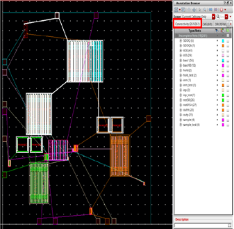
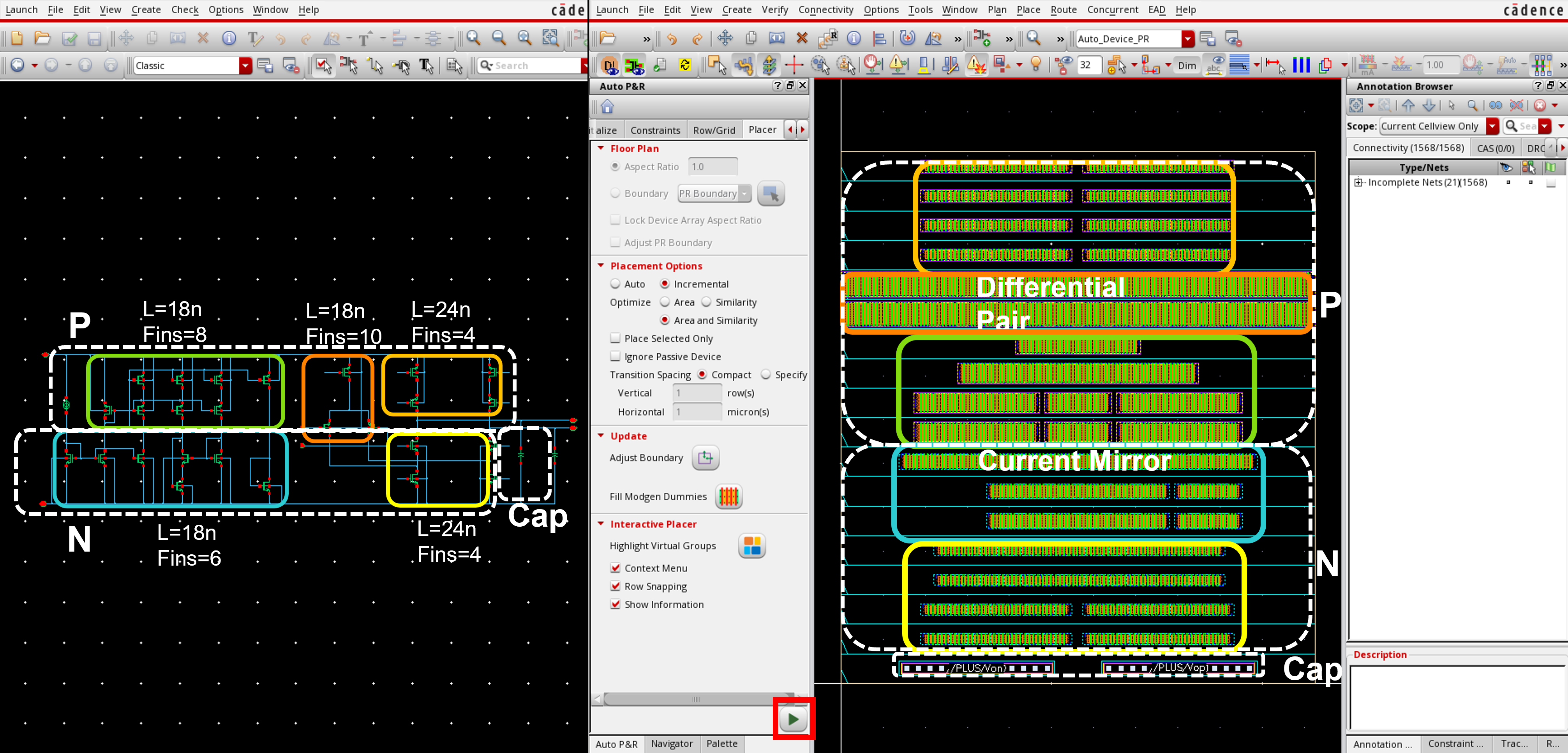
End-to-End ASIC & Custom IC Design Flow
Standardized custom IC workflow from schematic design and simulation to physical DRC/LVS and tape-out.
(Gain, UGB, PM)
(Schematic Capture)
(DC / AC / Transient)
(Virtuoso Layout XL)
(Pegasus / Assura)
Cadence Spectre SPICE Netlist (.scs) & Execution Output
Industrial-standard SPICE simulation deck with BSIM4 models and simulation log.
Spectre (R) Circuit Simulator -- Version 21.1.0.612.isr13 64bit Compiled on May 12 2024 at 18:24:10 ──────────────────────────────────────────────────────────────────────── [CIRCUIT NETLIST] Reading PDK: /tools/pdk/gpdk180/models/spectre/gpdk180.scs [DC OPERATION] Convergence achieved in 5 iterations: - M1/M2 Vds = 0.842 V | gm = 1.84 mS | Vgs - Vth = 142 mV (Sat) - Quiescent Current Idd = 420.5 uA | Total Power = 756.9 uW [AC ANALYSIS] Open-Loop Gain A0: 72.4 dB (Target > 65 dB) [PASSED] [AC ANALYSIS] Unity-Gain Bandwidth: 54.2 MHz (CL = 10 pF) [AC ANALYSIS] Phase Margin (PM): 65.4° (Target > 60°) [STABLE] [TRANSIENT] Slew Rate (SR+ / SR-): 48.2 V/us | Settling Time: 18.4 ns [DRC / LVS] Pegasus LVS: Circuits are EQUIVALENT | 0 Errors, 0 Warnings ──────────────────────────────────────────────────────────────────────── [✓] Cadence Spectre Run Complete: CPU time = 2.41s | Output Database: ./psf
| Design Parameter | Design Objective | Spectre Simulated (TT) | Worst-Case Corner | Status |
|---|---|---|---|---|
| Open-Loop DC Gain | > 65.0 dB | 72.4 dB | 68.1 dB (SS) | PASSED |
| Unity-Gain Bandwidth (UGB) | > 40.0 MHz | 54.2 MHz | 48.5 MHz (SF) | PASSED |
| Phase Margin (PM) | > 60.0° | 65.4° | 61.2° (FS) | STABLE |
| Total Power Dissipation | < 1.0 mW | 756.9 uW | 910.4 uW (FF) | OPTIMAL |
| Slew Rate (SR) | > 35 V/us | 48.2 V/us | 42.0 V/us (SS) | PASSED |