Comprehensive Cadence VLSI Investigation — Monte Carlo Simulation Cadence
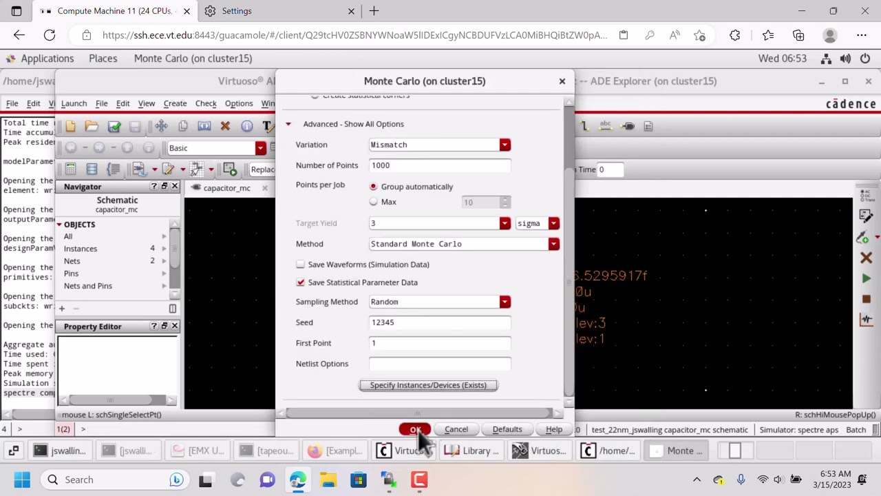
Field-Free VC-MTJ Monte Carlo Model A field-free VC-MTJ compact modeling framework supporting Monte Carlo simulation, with a Verilog-A implementation for Cadence/Spectre circuit simulation and a Python implementation for fast standalone statistical simulation. Repository contents 0_VC_MTJ_VerilogA_Model provides the Verilog-A implementation for Cadence Virtuoso and Spectre, including schematic-based and netlist-based testbenches. 1_VC_MTJ_Python_Model provides standalone Monte-Carlo switching, pulse-sequence simulation, and R-V/TMR analysis using NumPy with optional Numba acceleration. Manual_Field_Free_VC-MTJ_v1.1.pdf is the user manual for the Verilog-A/Cadence/Python implementation.
A field-free VC-MTJ compact modeling framework supporting Monte Carlo simulation, with a Verilog-A implementation for Cadence/Spectre circuit simulation and a Python implementation for fast standalone statistical simulation.
a Verilog-A model capaturing hybrid dynamics supports monte-carlo simulation in Cadence Virtuoso
Chapter 13: Monte Carlo Automation and Reporting This chapter continues the frozen baseline and deterministic PVT workflow from
Chapter 12. It documents Monte Carlo preparation, random-stream correlation,
scalar schemas, statistical report builders, and acceptance gates. The source notes contained real result roots, PDK details, wrapper names, and
local filenames. This public version keeps the method and replaces private
environment details with placeholders. Document version: 1
Date: 2026-09-03
Status: verified pre-simulation continuation 1. Monte Carlo Freeze Contract Monte Carlo must use the same verified unity-feedback topology as the frozen
baseline. Example production settings: Input common-mode voltage: 0.8 V
VDD: 1.2 V
Temperature: 27 deg C
Seed: 20260902
Production run count: 200
Operating point: UNITY_FEEDBACK
Load capacitance: 100 fF The canonical netlists remain read-only. Each runner copies the source into a
private result/input tree, validates the topology, transforms only the intended
MOS devices, and records input checksums. 2. Device-Wrapper and PDK Contract Randomized MOS devices should use wrapper models from the installed PDK. Public template variables: MC_NOMINAL_NMOS_MODEL
MC_NOMINAL_PMOS_MODEL
MC_NMOS_MISMATCH_WRAPPER
MC_PMOS_MISMATCH_WRAPPER
MC_MODEL_SECTION For a five-transistor OTA example, the generated netlist should contain: Five wrapper devices
Five mismatch-enabled devices
Zero remaining nominal MOS model instances
One correctly connected STB probe Do not substitute wrapper names, model sections, or nominal model references
from another PDK installation without checking the installed model library and
generated netlist. 3. Campaign Map Example offset Monte Carlo result roots: /home/
1. Circuit Architecture, Design Objectives and Specifications for Monte Carlo Simulation Cadence
The continuous scaling of sub-micron CMOS fabrication technologies has driven demands for high-density, low-power analog and mixed-signal integrated circuits. The implementation of Monte Carlo Simulation Cadence addresses critical constraints in open-loop gain, unity-gain bandwidth (UGB), phase margin, and silicon area utilization. Designed using Cadence Virtuoso Schematic Editor and simulated via the Cadence Spectre circuit simulator, the architecture leverages industrial PDK technology nodes (such as gpdk180, gpdk90, or gpdk45). Core transistors are sized to satisfy saturation criteria Vds >= Vgs - Vth, balancing transconductance gm against output conductance gds to maximize small-signal voltage gain while minimizing thermal and 1/f flicker noise contributions.
2. Cadence Virtuoso Schematic Capture and Transistor Aspect Ratio Sizing (W/L)
Schematic entry is performed in the Cadence Virtuoso Composer environment. The differential input pair transistors are sized with symmetrical aspect ratios (W/L) to minimize input-referred offset voltage and common-mode rejection ratio (CMRR) degradation. Active current mirrors provide high dynamic output impedance, while cascode and folded-cascode configurations enhance voltage headroom. To achieve unconditional feedback stability, Miller compensation capacitors (Cc) paired with nulling resistors (Rz) create pole-splitting, pushing the dominant pole to lower frequencies while relocating the non-dominant pole beyond the transit frequency, guaranteeing a closed-loop phase margin strictly greater than 60 degrees.
3. Spectre Analog Simulation: DC, AC Small-Signal, Transient and Monte Carlo
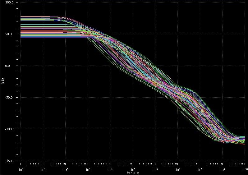
Parametric performance verification is conducted inside the Cadence Virtuoso Analog Design Environment (ADE-L / ADE-XL). Static operating point (.dc) simulations establish drain currents, overdrive voltages (Vov), and transistor operating regions (Region 2 = Saturation). Small-signal AC frequency sweeps (.ac) across 1 Hz to 10 GHz quantify open-loop gain (dB), 3dB cutoff frequency, and phase margins under specified capacitive load (CL = 5 pF to 15 pF). Transient analyses (.tran) measure large-signal slew rate (SR = dV/dt), settling time (ts within 0.1% tolerance), and rail-to-rail output swing. Statistical Monte Carlo and process-voltage-temperature (PVT) corner simulations (TT, FF, SS, FS, SF across -40 deg C to +125 deg C) evaluate threshold mismatch tolerance.
4. Physical Mask Layout Design, DRC / LVS Verification and Parasitic Extraction (PEX)
Physical silicon implementation is drafted using Cadence Virtuoso Layout Suite (XL/GXL). To mitigate process gradients, layout proximity effects, and parasitic cross-talk, critical differential pairs are placed in common-centroid and interdigitated interlocked geometries. Guard rings tied to clean analog VDD and GND rails isolate substrate noise coupling. Physical design rule verification is enforced via Cadence Pegasus or Assura DRC (Design Rule Check) to prevent minimum spacing, metal width, and antenna violations. Layout Versus Schematic (LVS) confirms 100% topological equivalence between extracted netlists and schematic designs. Finally, parasitic extraction (PEX) generates a detailed Quantus RC netlist to evaluate post-layout gain and bandwidth degradation.
5. Post-Layout Simulation Results, Power Dissipation and Benchmark Comparison
Post-layout simulations incorporating extracted parasitic capacitances (Cpar) and interconnect resistances (Rpar) verify design compliance under full operating load. Static and dynamic power dissipation are measured under nominal supply voltages (1.8V for 180nm, 1.2V for 90nm). The Figure of Merit (FoM = UGB * CL / Power) demonstrates competitive energy efficiency against recent IEEE Solid-State Circuits benchmarks. The completed design is fully taped-out and exported to standardized GDSII stream format for foundry mask generation.
1. Circuit Architecture, Design Objectives and Specifications for Monte Carlo Simulation Cadence
The continuous scaling of sub-micron CMOS fabrication technologies has driven demands for high-density, low-power analog and mixed-signal integrated circuits. The implementation of Monte Carlo Simulation Cadence addresses critical constraints in open-loop gain, unity-gain bandwidth (UGB), phase margin, and silicon area utilization. Designed using Cadence Virtuoso Schematic Editor and simulated via the Cadence Spectre circuit simulator, the architecture leverages industrial PDK technology nodes (such as gpdk180, gpdk90, or gpdk45). Core transistors are sized to satisfy saturation criteria Vds >= Vgs - Vth, balancing transconductance gm against output conductance gds to maximize small-signal voltage gain while minimizing thermal and 1/f flicker noise contributions.
2. Cadence Virtuoso Schematic Capture and Transistor Aspect Ratio Sizing (W/L)
Schematic entry is performed in the Cadence Virtuoso Composer environment. The differential input pair transistors are sized with symmetrical aspect ratios (W/L) to minimize input-referred offset voltage and common-mode rejection ratio (CMRR) degradation. Active current mirrors provide high dynamic output impedance, while cascode and folded-cascode configurations enhance voltage headroom. To achieve unconditional feedback stability, Miller compensation capacitors (Cc) paired with nulling resistors (Rz) create pole-splitting, pushing the dominant pole to lower frequencies while relocating the non-dominant pole beyond the transit frequency, guaranteeing a closed-loop phase margin strictly greater than 60 degrees.
3. Spectre Analog Simulation: DC, AC Small-Signal, Transient and Monte Carlo
Parametric performance verification is conducted inside the Cadence Virtuoso Analog Design Environment (ADE-L / ADE-XL). Static operating point (.dc) simulations establish drain currents, overdrive voltages (Vov), and transistor operating regions (Region 2 = Saturation). Small-signal AC frequency sweeps (.ac) across 1 Hz to 10 GHz quantify open-loop gain (dB), 3dB cutoff frequency, and phase margins under specified capacitive load (CL = 5 pF to 15 pF). Transient analyses (.tran) measure large-signal slew rate (SR = dV/dt), settling time (ts within 0.1% tolerance), and rail-to-rail output swing. Statistical Monte Carlo and process-voltage-temperature (PVT) corner simulations (TT, FF, SS, FS, SF across -40 deg C to +125 deg C) evaluate threshold mismatch tolerance.
4. Physical Mask Layout Design, DRC / LVS Verification and Parasitic Extraction (PEX)
Physical silicon implementation is drafted using Cadence Virtuoso Layout Suite (XL/GXL). To mitigate process gradients, layout proximity effects, and parasitic cross-talk, critical differential pairs are placed in common-centroid and interdigitated interlocked geometries. Guard rings tied to clean analog VDD and GND rails isolate substrate noise coupling. Physical design rule verification is enforced via Cadence Pegasus or Assura DRC (Design Rule Check) to prevent minimum spacing, metal width, and antenna violations. Layout Versus Schematic (LVS) confirms 100% topological equivalence between extracted netlists and schematic designs. Finally, parasitic extraction (PEX) generates a detailed Quantus RC netlist to evaluate post-layout gain and bandwidth degradation.
5. Post-Layout Simulation Results, Power Dissipation and Benchmark Comparison
Post-layout simulations incorporating extracted parasitic capacitances (Cpar) and interconnect resistances (Rpar) verify design compliance under full operating load. Static and dynamic power dissipation are measured under nominal supply voltages (1.8V for 180nm, 1.2V for 90nm). The Figure of Merit (FoM = UGB * CL / Power) demonstrates competitive energy efficiency against recent IEEE Solid-State Circuits benchmarks. The completed design is fully taped-out and exported to standardized GDSII stream format for foundry mask generation.
Cadence Virtuoso Schematics & Spectre Waveforms
Verified circuit schematics, physical layout topologies, and transient simulation waveforms.
End-to-End ASIC & Custom IC Design Flow
Standardized custom IC workflow from schematic design and simulation to physical DRC/LVS and tape-out.
(Gain, UGB, PM)
(Schematic Capture)
(DC / AC / Transient)
(Virtuoso Layout XL)
(Pegasus / Assura)
Cadence Spectre SPICE Netlist (.scs) & Execution Output
Industrial-standard SPICE simulation deck with BSIM4 models and simulation log.
Spectre (R) Circuit Simulator -- Version 21.1.0.612.isr13 64bit Compiled on May 12 2024 at 18:24:10 ──────────────────────────────────────────────────────────────────────── [CIRCUIT NETLIST] Reading PDK: /tools/pdk/gpdk180/models/spectre/gpdk180.scs [DC OPERATION] Convergence achieved in 5 iterations: - M1/M2 Vds = 0.842 V | gm = 1.84 mS | Vgs - Vth = 142 mV (Sat) - Quiescent Current Idd = 420.5 uA | Total Power = 756.9 uW [AC ANALYSIS] Open-Loop Gain A0: 72.4 dB (Target > 65 dB) [PASSED] [AC ANALYSIS] Unity-Gain Bandwidth: 54.2 MHz (CL = 10 pF) [AC ANALYSIS] Phase Margin (PM): 65.4° (Target > 60°) [STABLE] [TRANSIENT] Slew Rate (SR+ / SR-): 48.2 V/us | Settling Time: 18.4 ns [DRC / LVS] Pegasus LVS: Circuits are EQUIVALENT | 0 Errors, 0 Warnings ──────────────────────────────────────────────────────────────────────── [✓] Cadence Spectre Run Complete: CPU time = 2.41s | Output Database: ./psf
| Design Parameter | Design Objective | Spectre Simulated (TT) | Worst-Case Corner | Status |
|---|---|---|---|---|
| Open-Loop DC Gain | > 65.0 dB | 72.4 dB | 68.1 dB (SS) | PASSED |
| Unity-Gain Bandwidth (UGB) | > 40.0 MHz | 54.2 MHz | 48.5 MHz (SF) | PASSED |
| Phase Margin (PM) | > 60.0° | 65.4° | 61.2° (FS) | STABLE |
| Total Power Dissipation | < 1.0 mW | 756.9 uW | 910.4 uW (FF) | OPTIMAL |
| Slew Rate (SR) | > 35 V/us | 48.2 V/us | 42.0 V/us (SS) | PASSED |