Enquire Now
Medical Computer Vision · Clinical Diagnostics · PyTorch / TensorFlow · GPU Optimized · 2026

Skin Cancer Classification Cnn Capstone Project

Tensor Pipeline · Custom Loss Formulations · Model Quantization · Accelerated Inference — A rigorous deep learning engineering project focused on automated pathological lesion segmentation and radiological disease classification. Architected for thesis defense viva presentations, IEEE reproduction, and high-throughput production deployment.

PyTorch
Core Framework
AMP FP16
Mixed Precision
TensorRT
Quantized Serving

1

Abstract— Recently, there has been great interest in developing Artificial Intelligence (AI) enabled computer-aided diagnostics solutions for the diagnosis of skin cancer. With the increasing incidence of skin cancers, low awareness among a growing population, and a lack of adequate clinical expertise and services, there is an immediate need for AI systems to assist clinicians in this domain. A large number of skin lesion datasets are available publicly, and researchers have developed AI solutions, particularly deep learning algorithms, to distinguish malignant skin lesions from benign lesions in different image modalities such as dermoscopic, clinical, and histopathology images. Despite the various claims of AI systems achieving higher accuracy than dermatologists in the classification of different skin lesions, these AI systems are still in the very early stages of clinical application in terms of being ready to aid clinicians in the diagnosis of skin cancers. In this review, we discuss advancements in the digital image-based AI solutions for the diagnosis of skin cancer, along with some challenges and future opportunities to improve these AI systems to support dermatologists and enhance their ability to diagnose skin cancer.

skin cancer classification cnn capstone project Diagram
Figure: System Model & Simulation Flow for Skin Cancer Classification Cnn Capstone Project

Index Terms—Skin Cancer, Artificial Intelligence, Deep Learning, Dermatologists, Computer-aided Diagnostics, Digital Dermatology.

skin cancer classification cnn capstone project Diagram
Figure: System Model & Simulation Flow for Skin Cancer Classification Cnn Capstone Project

I. Introduction

According to the Skin Cancer Foundation, the global incidence of skin cancer continues to increase . In 2019, it is estimated that 192,310 cases of melanoma will be diagnosed in the United States . However, the most common forms of skin cancer are non-melanocytic, such as Basal Cell Carcinoma (BCC) and Squamous Cell Carcinoma (SCC). Non-melanoma skin cancer is the most commonly occurring cancer in men and women, with over 4.3 million cases of BCC and 1 million cases of SCC diagnosed each year in the United States, although these numbers are likely to be an underestimate . Early diagnosis of skin cancer is a cornerstone to improving outcomes and is correlated with 99% overall survival (OS). However, once disease progresses beyond the skin, survival is poor , .

skin cancer classification cnn capstone project Diagram
Figure: System Model & Simulation Flow for Skin Cancer Classification Cnn Capstone Project

Nh, Usa.

In current medical practice, dermatologists examine patients by visual inspection with the assistance of polarized light magnification via dermoscopy. Medical diagnosis often depends on the patient’s history, ethnicity, social habits and exposure to the sun. Lesions of concern are biopsied in an office setting, submitted to the laboratory, processed as permanent paraffin sections, and examined as representative glass slides by a pathologist to render a diagnosis.

AI-enabled computer-aided diagnostics (CAD) solutions are poised to revolutionize medicine and health care, especially in medical imaging. Medical imaging, including ultrasound, computed tomography (CT), and magnetic resonance imaging (MRI), is used extensively in clinical practice. In the dermatological realm, dermoscopy or, less frequently, confocal microscopy, allows for more detailed in vivo visualization of lesioned features and risk stratification , , , , . In various studies, AI algorithms match or exceed clinician performance for disease detection in medical imaging , . Recently, deep learning has provided various end-to-end solutions in the detection of abnormalities such as breast cancer, brain tumors, lung cancer, esophageal cancer, skin lesions, and foot ulcers across multiple image modalities of medical imaging , , , , .

Over the last decade, advances in technology have led to greater accessibility to advanced imaging techniques such as 3D whole body photoimaging/scanning, dermoscopy, high- resolution cameras, and whole-slide digital scanners that are used to collect high-quality skin cancer data from patients across the world , . The International Skin Imaging Collaboration (ISIC) is a driving force that provides digital datasets of skin lesion images with expert annotations for automated CAD solutions for the diagnosis of melanoma and other skin cancers. A wide research interest in AI solutions for skin cancer diagnosis is facilitated by affordable and highspeed internet, computing power, and secure cloud storage to manage and share skin cancer datasets. These algorithms can be scalable to multiple devices, platforms, and operating systems, turning them into modern medical instruments .

The purpose of this review is to provide the reader with an update on the performance of artificial intelligence algorithms Medicine, Dartmouth-Hitchcock Medical Center, Geisel School of Medicine, Dartmouth College, Hanover, NH, USA.

Epidemiology, Dartmouth College, Hanover, NH, USA.

Challenges And Opportunities

Manu Goyal1, Thomas Knackstedt2, Shaofeng Yan3, and Saeed Hassanpour4

2

used for the diagnosis of skin cancer across various modalities of skin lesion datasets, especially in terms of the comparative

And

dermatologists/ dermatopathologists. We dedicated separate sub-sections to arrange these studies according to the types of imaging modality used, including clinical photographs, dermoscopy images, and whole-slide pathology scanning.

Specifically, we seek to discuss the technical challenges in this domain and opportunities to improve the current AI solutions so that they can be used as a support tool for clinicians to enhance their efficiency in diagnosing skin cancers.

Ii. Artificial Intelligence For Skin Cancer

The major advances in this field came from the work of Esteva et al. who used a deep learning algorithm on a combined skin dataset of 129,450 clinical and dermoscopic images consisting of 2,032 different skin lesion diseases. They compared the performance of a deep learning method with 21

And

differentiation of carcinomas versus benign seborrheic keratoses; and melanomas versus benign nevi. The performance of AI was demonstrated to be on par with dermatologists’ performance for skin cancer classification. Three main types of modalities are used for the skin lesion classification and diagnosis in the work described here: clinical images, dermoscopic images, and histopathology images. In this section, we start with analysis of publicly available skin lesion datasets, and then we provide different sub-sections dedicated to the artificial intelligence solution related to each type of imaging modality.

A. Publicly Available Datasets For Skin Cancer

1) ISIC Archive: The ISIC archive gallery consists of many clinical and dermoscopic skin lesion datasets from across the world, such as ISIC Challenges datasets , HAM10000 , and BCN20000 .

2) Interactive Atlas of Dermoscopy : The Interactive Atlas of Dermoscopy has 1,000 clinical cases (270 melanomas, 49 seborrheic keratoses), each with at least two images: dermoscopic, and close-up clinical. It is available for research purposes and has a fee of €250.

3) Dermofit Image Library : The Dermofit Image Library consists of 1,300 high-resolution images with 10 classes of skin lesions. There is a need for a licensing agreement with a one- off license fee of €75, and an academic license is available.

4) PH2 Dataset : The PH2 Dataset has 200 dermoscopic images (40 melanoma and 160 nevi cases). It is freely available after signing a short online registration form.

6) MED-NODE Dataset : It consists of 170 clinical images (70 melanoma and 100 nevi cases). This dataset is freely available to download for research.

7) Asan Dataset , : It is a collection of 17,125 clinical images of 12 types of skin diseases found in Asian people. The Asan Test Dataset (1,276 images) is available to download for research.

8) Hallym Dataset : This dataset consists of 125 clinical images of BCC cases. 9) SD-198 Dataset : The SD-198 dataset is a clinical skin lesion dataset containing 6,584 clinical images of 198 skin diseases. This dataset was captured with digital cameras and mobile phones.

10) SD-260 Dataset : This dataset is a more balanced dataset when compared to the previous SD-198 dataset since it controls the class size distribution with preservation of 10–60 images for each category. It consists of 20,600 images with 260 skin diseases.

11) Dermnet NZ : Dermnet NZ has one of the largest and most diverse collections of clinical, dermoscopic and histology images of various skin diseases. These images can be used for academic research purposes. They have additional high- resolution images for purchase.

12) Derm7pt : This dataset has around 2,000 dermoscopic and clinical images of skin lesions, with a 7-point check-list criteria.

13) The Cancer Genome Atlas : This dataset is one of the largest collections of pathological skin lesion slides with 793 cases. It is publicly available for the research community to use.

B. Artificial Intelligence In Dermoscopic Images

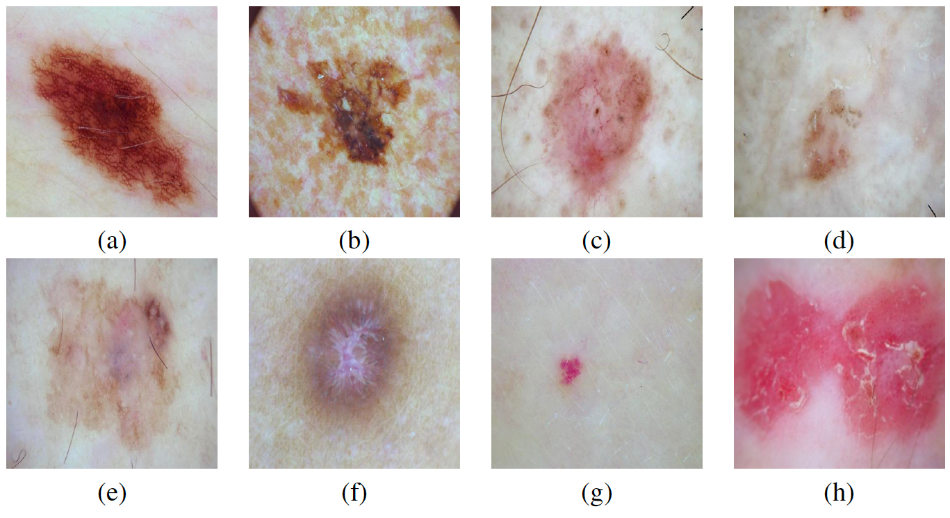
Dermoscopy is the inspection/examination of skin lesions with a dermatoscope device consisting of a high-quality magnifying lens and a (polarizable) illumination system. Dermoscopic images are captured with high-resolution digital single-lens reflex (DSLR) or smartphone camera attachments. The use of dermoscopic images for AI algorithms is becoming a very popular research field since the introduction of many large publicly available dermoscopic datasets consisting of different types of benign and cancerous skin lesions, as shown in Fig. 1.

There have been multiple AI studies on lesion diagnosis using dermoscopic skin lesion datasets, which are listed below. Fig. 1. Illustration of different types of dermoscopic skin lesions where (a) Nevi (b) Melanoma (c) Basal Cell Carcinoma (d) Actinic Keratosis (e) Benign Keratosis (f) Dermatofibroma (g) Vascular Lesion (h) Squamous Cell

1) Codella Et Al. Developed An Ensemble Of Deep

learning algorithms on the ISIC-2016 dataset and compared the performance of this network with 8 dermatologists for the classification of 100 skin lesions as benign or malignant. The ensemble method outperformed the average performance of dermatologists by achieving an accuracy of 76% and specificity of 62% versus 70.5% and 59% achieved by dermatologists.

2) Haenssle et al. trained a deep learning method InceptionV4 on a large dermoscopic dataset consisting of more than 100,000 benign lesions and melanoma images and

3

compared the performance of a deep learning method with 58 dermatologists. On the test set of 100 cases (75 benign lesions and 25 melanoma cases), dermatologists had an average sensitivity of 86.6% and specificity of 71.3%, while the deep learning method achieved a sensitivity of 95% and specificity of 63.8%.

3) Brinker et al. compared the performance of 157 hospitals with a deep learning method (ResNet50) for 100 dermoscopic images (MClass-D) consisting of 80 nevi and 20 melanoma cases. Dermatologists achieved an overall sensitivity of 74.1%, and specificity of 60.0% on the dermoscopic dataset whereas a deep learning method achieved a specificity of 69.2% and a sensitivity of 84.2%.

4) Tschandl Et Al. Used Popular Deep Learning

architectures known as InceptionV3 and ResNet50 on a combined dataset of 7,895 dermoscopic and 5,829 close-up lesion images for diagnosis of non-pigmented skin cancers.

The performance is compared with 95 dermatologists divided into three groups based on experience. The deep learning algorithms achieved accuracy on par with human experts and exceeded the human groups with beginner and intermediate raters.

5) Maron Et Al. Compared The Sensitivity And

specificity of a deep learning method (ResNet50) with 112 German dermatologists for multiclass classification of skin lesions which includes nevi, melanoma, benign keratosis, BCC, and SCC (also solar keratosis and intraepithelial

Carcinoma). The Deep Learning Method Outperformed

dermatologists at a significant level (p ≤ 0.001).

6) Haenssle Et Al. Compared The Deep Learning

architecture based on InceptionV4 (approved as medical

Device By European Union) And Dermatologists On A

dermoscopic test set consists of 100 cases (60 benign and 40 malignant lesions). This study was performed on two levels i.e. level I: dermoscopic image; level II: additional clinical

Information. The Deep Learning Algorithm Achieved

sensitivity and specificity score of 95% and 76.7% respectively, whereas, mean sensitivity and specificity of 89% and 80.7% respectively achieved by dermatologists in level I. With more information in level II, the mean sensitivity of dermatologists increased to 94.1% whereas mean specificity remained same.

7) Tschandl Et Al. Compared The Average

performance of both AI algorithms (139 in total) participated in the ISIC 2018 challenge and 511 human readers on a test set of 1511 images. In results, the AI algorithms achieved more correct diagnosis than human readers.

C. Artificial Intelligence In Clinical Images

Clinical images are routinely captured of different skin lesions with mobile cameras for remote examination and incorporation into patient medical records, as shown in Fig. 2. Since clinical images are captured with different cameras with variable backgrounds, illuminance and color, these images provide different insights for dermoscopic images.

1) Yang Et Al. Performed Clinical Skin Lesion

diagnosis using representation inspired by the ABCD rule on the SD-198 dataset. They compared the performance of the

Proposed Methods With Deep Learning Methods And

dermatologists. It achieved a score of 57.62% (accuracy) in comparison to the best performing deep learning method (ResNet), which achieved 53.35%. When compared to the clinicians, only senior clinicians who have considerable experience in skin disease achieved an average accuracy of 83.29%.

2) Han et al. trained a deep learning architecture (ResNet-152) to classify the clinical images of 12 skin diseases on an Asan training dataset, a MED-NODE dataset, and atlas site images, and tested it on an Asan testing set and

An Edinburgh Dataset (Dermofit). The Algorithm’S

performance was on par with the team of 16 dermatologists on 480 randomly chosen images from the Asan test dataset (260 images) and the Edinburgh dataset (220 images), whereas the AI system outperformed dermatologists in the diagnosis of BCC.

3) Fujisawa et al. tested a deep learning method on 6,009 clinical images of 14 diagnoses, including both malignant and benign conditions. The deep learning algorithm achieved a diagnostic accuracy of 76.5% which is superior to the performance of 13 board-certified dermatologists (59.7%) and nine dermatology trainees (41.7%) on a 140-image dataset.

4) Brinker et al. compared the performance of 145 dermatologists and a deep learning method (ResNet50) for the test case of 100 clinical skin lesion images (MClass-ND) consisting of 80 nevi cases and 20 biopsy-verified melanoma cases. The dermatologists achieved an overall sensitivity of 89.4%, a specificity of 64.4% and an AUROC of 0.769

Whereas A Deep Learning Method Achieved The Same

sensitivity and better specificity score of 69.2%. Fig. 2. Illustration of different types of clinical skin lesions where (a) Benign

Keratosis (B) Melanoma (C) Bcc (D) Scc

D. Artificial Intelligence in Histopathology Images

By

dermatopathologists based on microscopic evaluation of a tissue biopsy. Deep learning solutions have been successful in the field of digital pathology with whole-slide imaging.

Examples of histopathology images of skin lesions are shown in Fig. 3. These techniques are used for the classification of biopsy tissue specimens to diagnose the number of cancers such as skin, lung, and breast. In this section, we explore the deep learning methods used in digital histopathology specific to skin cancer.

1) Heckler Et Al. Used A Deep Learning Method

(ResNet50) to compare the performance of pathologists in classifying melanoma and nevi. The deep learning model was trained on a dataset of 595 histopathology images (300

Melanoma And 295 Nevi) And Tested On 100 Images

(melanoma/nevi = 1:1). The total discordance with the histopathologist was 18% for melanoma, 20% for nevi, and 19% for the full set of images.

2) Jiang et al. proposed the use of a deep learning algorithm on smartphone-captured digital histopathology images (MOI) for the detection of BCC. They found that the performance of the algorithm on MOI and Whole Slide Imaging (WSI) is comparable with an AUC score of 0.95.

They introduced a deep segmentation network for in-depth analysis of the hard cases to further improve the performance with 0.987 (AUC), 0.97 (sensitivity), 0.94 (specificity) score.

3. Cruz-Roa et al. used a deep learning architecture to discriminate between BCC and normal tissue patterns on 1,417 images from 308 Region of Interests (ROI) of skin histopathology images. They compared the deep learning method with traditional machine learning with feature descriptors, including the bag of features, canonical and Haar- based wavelet transform. The deep learning architecture proved superior over the traditional approaches by achieving 89.4% in F-Measure and 91.4% in balanced accuracy.

4) Xie et al. introduced a large dataset of 2,241 histopathological images of 1,321 patients from 2008 to 2018. They used two deep learning architectures, VGG19 and ResNet50, on the 9.95 million patches generated on 2,241 histopathological images to test the classification of melanoma and nevi on different magnification scales. They achieved high accuracy in distinguishing melanoma from nevi with average F1 (0.89), Sensitivity (0.92), Specificity (0.94) and AUC (0.98).

Fig. 3. Illustration of different types of histopathology images where (a) Nevi (b) Melanoma (c) Basal Cell Carcinoma (d) Squamous Cell Carcinoma

Iii. Challenges In Artificial Intelligence

With deep learning algorithms surpassing the benchmarks of popular computer vision datasets in a short period, the same trend could be expected in the skin lesion diagnosis challenge as well. However, as we further explore the skin lesion diagnosis challenge, this task appears to be not straightforward like ImageNet, PASCAL-VOC, MS-COCO challenges in a

Non-Medical Domain , . There Are Intra-Class

similarities and inter-class dissimilarities regarding color, texture, size, place, and appearance in the visual appearance of skin lesions. Deep learning algorithms generally require a substantial amount of diverse, balanced, and high-quality training data that represent each class of skin lesions to improve diagnostic accuracy. For skin lesion datasets of various modalities, there are many more issues related to the diagnosis of skin cancer with AI solutions as discussed below.

A. Performance of Deep Learning and Unbalanced Datasets The performance of deep learning algorithms mostly depends on the quality of image datasets rather than tuning the hyper- parameters of networks, as is commonly seen in the different publicly available skin lesion datasets. There are generally more cases of benign skin lesions rather than malignant lesions. Most of the deep learning architectures are designed on a balanced dataset, such as ImageNet, which consists of 1,000 images per class (1000 classes) . Hence, the performance of a deep learning algorithm usually suffers from unbalanced datasets, despite using tuning tricks like a penalty for false negatives found in minor skin lesion classes during training using custom loss functions.

B. Curious Case of Histopathology Images/ Digital Pathology The size of images in clinical and dermoscopic skin lesion datasets varies between 1200 × 768 and 3648 × 2736 depending on the camera used. Most of the deep learning algorithms are usually developed and validated on large datasets of non- medical background. These deep learning algorithms have worked very well on clinical and dermoscopic skin lesion datasets by fine tuning the algorithms through transfer learning techniques. On the other hand, histopathological scans consist of millions of pixels and their dimensions are commonly larger than 50,000 x 50,000. Hence, there are many technical challenges for deep learning or AI algorithms in digital pathology such as lack of labeled data, infinite pattern from different types of tissues, high-quality feature extraction, high computational expenses and many more .

C. Patients’ Medical History and Clinical Meta-data Patients’ medical history, social habits, and clinical meta- data are considered when making a skin cancer diagnosis. It is very important to know the diagnostic meta-data, such as patient and family history of skin cancer, age, ethnicity, sex, general anatomic site, size and structure of the skin lesion, while performing a visual inspection of a suspected skin lesion with dermoscopy. Hence, only image-based deep learning algorithms used for the diagnosis of skin cancer falter on key aspects of patient and clinical information. It is proven in a previous study that both ‘beginners’ and ‘skilled’ dermatologists’ performance is improved with the availability of clinical information and that they performed better than deep learning algorithms. Unfortunately, both patient history and clinical meta-data are missing in the most publicly available skin lesion datasets.

D. Abcde Rule And Time-Line Datasets

In the clinical setting, a suspicious lesion is visually inspected with the help of dermoscopy. The ABCDE rule is considered an important rule for differentiating benign moles (nevi) from melanoma. This includes whether the lesion is asymmetrical, has irregular borders, displays multiple colors, whether the diameter of the lesion is greater than six millimetres, and if there has been any evolution or change in the composition of the lesion. Despite the availability of

Ai Adaptive Learning

This project focuses on ai adaptive learning using modern AI and machine learning techniques. The content below is adapted from research literature and practical implementation notes.

We propose a novel high-performance and interpretable canon-

addition, unlike tree learning, DNNs enable gradient descent- ical deep tabular data learning architecture, TabNet. TabNet based end-to-end learning for tabular data which can have a uses sequential attention to choose which features to reason multitude of benefits: (i) efficiently encoding multiple data from at each decision step, enabling interpretability and more types like images along with tabular data; (ii) alleviating the efficient learning as the learning capacity is used for the most need for feature engineering, which is currently a key aspect

salient features. We demonstrate that TabNet outperforms in tree-based tabular data learning methods; (iii) learning other variants on a wide range of non-performance-saturated from streaming data and perhaps most importantly (iv) end- tabular datasets and yields interpretable feature attributions to-end models allow representation learning which enables plus insights into its global behavior. Finally, we demonstrate many valuable application scenarios including data-efficient

self-supervised learning for tabular data, significantly improv- domain adaptation (Goodfellow, Bengio, and Courville 2016), ing performance when unlabeled data is abundant. generative modeling (Radford, Metz, and Chintala 2015) and

Introduction We propose a new canonical DNN architecture for tabular

Deep neural networks (DNNs) have shown notable success data, TabNet. The main contributions are summarized as: efficiently encode the raw data into meaningful representa- enabling flexible integration into end-to-end learning. tions, fuel the rapid progress. One data type that has yet to 2. TabNet uses sequential attention to choose which fea- see such success with a canonical architecture is tabular data. tures to reason from at each decision step, enabling in-

Despite being the most common data type in real-world AI terpretability and better learning as the learning capacity (as it is comprised of any categorical and numerical features), is used for the most salient features (see Fig. 1). This under-explored, with variants of ensemble decision trees for each input, and unlike other instance-wise feature se- Why? First, because DT-based approaches have certain bene- and van der Schaar 2019), TabNet employs a single deep

fits: (i) they are representionally efficient for decision mani- learning architecture for feature selection and reasoning. folds with approximately hyperplane boundaries which are 3. Above design choices lead to two valuable properties: (i) common in tabular data; and (ii) they are highly interpretable TabNet outperforms or is on par with other tabular learn- in their basic form (e.g. by tracking decision nodes) and there ing models on various datasets for classification and re-

are popular post-hoc explainability methods for their ensem- gression problems from different domains; and (ii) TabNet ble form, e.g. (Lundberg, Erion, and Lee 2018) – this is an enables two kinds of interpretability: local interpretability important concern in many real-world applications; (iii) they that visualizes the importance of features and how they are fast to train. Second, because previously-proposed DNN are combined, and global interpretability which quantifies

architectures are not well-suited for tabular data: e.g. stacked the contribution of each feature to the trained model. convolutional layers or multi-layer perceptrons (MLPs) are 4. Finally, for the first time for tabular data, we show signif- vastly overparametrized – the lack of appropriate inductive icant performance improvements by using unsupervised bias often causes them to fail to find optimal solutions for tab- pre-training to predict masked features (see Fig. 2).

ular decision manifolds (Goodfellow, Bengio, and Courville

Why is deep learning worth exploring for tabular data?

One obvious motivation is expected performance improve- Feature selection: Feature selection broadly refers to judi- Copyright © 2021, Association for the Advancement of Artificial ciously picking a subset of features based on their useful-

Professional occupation related Investment related

Feedback from Feedback to

Feature selection Input processing Feature selection Input processing

previous step next step … …

Predicted output (whether the income level >$50k)

selection enables interpretability and better learning as the capacity is used for the most salient features. TabNet employs multiple decision blocks that focus on processing a subset of input features for reasoning. Two decision blocks shown as examples process features that are related to professional occupation and investments, respectively, in order to predict the income level.

Unsupervised pre-training Supervised fine-tuning

Age Cap. gain Education Occupation Gender Relationship Age Cap. gain Education Occupation Gender Relationship 5 2000 ? Exec-managerial F Wife 6 2000 Bachelors Exec-managerial M Husband 1 0 ? Farming-fishing M ? 2 0 High-school Farming-fishing M Unmarried

? 50 Doctorate Prof-specialty M Husband 4 50 Doctorate Prof-specialty M Husband 2 ? ? Handlers-cleaners F Wife 2 0 High-school Handlers-cleaners F Wife 5 3000 Bachelors ? ? Husband 5 3000 Bachelors Exec-managerial M Husband

3 0 Bachelors ? F ? 3 100 Bachelors Prof-specialty F Wife ? 0 High-school Armed-Forces ? Husband 2 0 High-school Armed-Forces M Husband

TabNet decoder Decision making

Age Cap. gain Education Occupation Gender Relationship Income > $50k

3 M False

level can be guessed from the occupation, or the gender can be guessed from the relationship. Unsupervised representation learning by masked self-supervised learning results in an improved encoder model for the supervised learning task.

ward selection and Lasso regularization (Guyon and Elisseeff performance with compact representations. 2003) attribute feature importance based on the entire training Tree-based learning: DTs are commonly-used for tabular data, and are referred as global methods. Instance-wise fea- data learning. Their prominent strength is efficient picking ture selection refers to picking features individually for each of global features with the most statistical information gain

to maximize the mutual information between the selected mance of standard DTs, one common approach is ensembling features and the response variable, and in (Yoon, Jordon, and to reduce variance. Among ensembling methods, random van der Schaar 2019) by using an actor-critic framework to forests (Ho 1998) use random subsets of data with randomly mimic a baseline while optimizing the selection. Unlike these, selected features to grow many trees. XGBoost (Chen and

sity in end-to-end learning – a single model jointly performs recent ensemble DT approaches that dominate most of the feature selection and output mapping, resulting in superior recent data science competitions. Our experimental results

!# + Softmax !" < % !" > % !# > & !# > &

ReLU ReLU &

$" !" − $" % −1 −$" !" + $" % −1 −1 $# !# − $# & % −1 −$# !# + $# & !"

FC FC

W: [$" , - $" , 0, 0] W: [0, 0, $# , - $# ] !" < % b: [-a $" , a $" , -1, -1] b: [-1, -1, -d $# , d $# ] !# < & !" > % !# < & [!" ] [!# ]

M: [1, 0] M: [0, 1]

(right). Relevant features are selected by using multiplicative sparse masks on inputs. The selected features are linearly transformed, and after a bias addition (to represent boundaries) ReLU performs region selection by zeroing the regions. Aggregation of multiple regions is based on addition. As C and C get larger, the decision boundary gets sharper.

for various datasets show that tree-based models can be out- constructs a sequential multi-step architecture, where each performed when the representation capacity is improved with step contributes to a portion of the decision based on the deep learning while retaining their feature selecting property. selected features; (iii) improves the learning capacity via non- Integration of DNNs into DTs: Representing DTs with linear processing of the selected features; and (iv) mimics

DNN building blocks as in (Humbird, Peterson, and McClar- ensembling via higher dimensions and more steps. ren 2018) yields redundancy in representation and ineffi- cient learning. Soft (neural) DTs (Wang, Aggarwal, and Liu Fig. 4 shows the TabNet architecture for encoding tabu- functions, instead of non-differentiable axis-aligned splits. mapping of categorical features with trainable embeddings.

However, losing automatic feature selection often degrades We do not consider any global feature normalization, but performance. In (Yang, Morillo, and Hospedales 2018), a soft merely apply batch normalization (BN). We pass the same D- binning function is proposed to simulate DTs in DNNs, by dimensional features f ∈ <B×D to each decision step, where 2019) proposes a DNN architecture by explicitly leveraging multi-step processing with Nsteps decision steps. The ith

expressive feature combinations, however, learning is based step inputs the processed information from the (i − 1)th step on transferring knowledge from gradient-boosted DT. (Tanno to decide which features to use and outputs the processed ing from primitive blocks while representation learning into sion. The idea of top-down attention in the sequential form edges, routing functions and leaf nodes. TabNet differs from is inspired by its applications in processing visual and text

these as it embeds soft feature selection with controllable data (Hudson and Manning 2018) and reinforcement learn- Self-supervised learning: Unsupervised representation relevant information in high dimensional input. learning improves supervised learning especially in small Feature selection: We employ a learnable mask M[i] ∈ has shown significant advances – driven by the judicious capacity of a decision step is not wasted on irrelevant

choice of the unsupervised learning objective (masked input ones, and thus the model becomes more parameter effi- prediction) and attention-based deep learning. cient. The masking is multiplicative, M[i] · f . We use an attentive transformer (see Fig. 4) to obtain the masks us- TabNet for Tabular Learning ing the processed features from the preceding step, a[i − 1]:

M[i] = sparsemax(P[i − 1] · hi (a[i − 1])). Sparsemax nor-

DTs are successful for learning from real-world tabular malization (Martins and Astudillo 2016) encourages sparsity datasets. With a specific design, conventional DNN building by mapping the Euclidean projection onto the probabilistic blocks can be used to implement DT-like output manifold, simplex, which is observed to be superior in performance and e.g. see Fig. 3). In such a design, individual feature selec- aligned with the goal of sparse feature selection for explain-

tion is key to obtain decision boundaries in hyperplane form, PD which can be generalized to a linear combination of features ability. Note that j=1 M[i]b,j = 1. hi is a trainable func- where coefficients determine the proportion of each feature. tion, shown in Fig. 4 using a FC layer, followed by BN. P[i] TabNet is based on such functionality and it outperforms DTs is the prior scale term, denoting how much a particular feature

Qi while reaping their benefits by careful design which: (i) uses has been used previously: P[i] = j=1 (γ − M[j]), where γ sparse instance-wise feature selection learned from data; (ii) is a relaxation parameter – when γ = 1, a feature is enforced

+ Softmax

Feature Feature …

transformer transformer

x Nsteps Features

+ Softmax

Feature …

transformer transformer Feature Feature Feature Feature transformer

Encoded representation

transformer transformer Attentive transformer … Mask transformer …

Step 2 Decision step dependent

transformer transformer

BN Feature Feature

FC BN transformer transformer

+ 0.5 0.5 0.5 Agg. Agg. Features Features FC FC + +

Reconstructed + … Feature attributes + … features

(a) TabNet encoder architecture (b) TabNet decoder architecture Feature transformer Feature Attentive transformer Shared across decision steps Decision step dependent transformer GLU

Decision step dependent Prior scales

+ 0.5 0.5 0.5

0.5 0.5 0.5

+ Attentive transformer (c) (d)

Prior scales

divides the processed representation to be used by the attentive transformer of the subsequent step as well as for the overall Attentive BN FC

output. For each step, the feature selection mask provides interpretable information about the model’s functionality, and the +

masks can be aggregated to obtain global feature transformer important attribution. (b) TabNet decoder, composed of a feature transformer block at each step. (c) A feature transformer block example – 4-layer network is shown, where 2 are shared across all decision

Prior scales

steps and 2 are decision step-dependent. Each layer is composed of a fully-connected (FC) layer, BN and GLU nonlinearity. (d) +

An attentive transformer block example – a single layer mapping is modulated with a prior scale information which aggregates Sparsemax

how much each feature has been used before the current decision step. sparsemax (Martins and Astudillo 2016) is used for BN FC

normalization of the coefficients, resulting in sparse selection of the salient features. +

to be used only at one decision step and as γ increases, more propose the aggregate.feature importance mask, Magg−b,j = flexibility is provided to use a feature at multiple decision PNsteps ηb [i]Mb,j [i]

PD PNsteps

ηb [i]Mb,j [i].2 i=1 i=1 steps. P is initialized as all ones, 1B×D , without any prior j=1

on the masked features. If some features are unused (as in self- Tabular self-supervised learning: We propose a decoder supervised learning), corresponding P entries are made 0 architecture to reconstruct tabular features from the Tab- to help model’s learning. To further control the sparsity of the Net encoded representations. The decoder is composed of selected features, we propose sparsity regularization in the feature transformers, followed by FC layers at each deci-

form of entropy (Grandvalet and Bengio 2004), Lsparse = sion step. The outputs are summed to obtain the recon-

PNsteps PB PD −Mb,j [i] log(Mb,j [i]+)

i=1 b=1 j=1 Nsteps ·B , where  is a structed features. We propose the task of prediction of miss- small number for numerical stability. We add the sparsity reg- ing feature columns from the others. Consider a binary mask ularization to the overall loss, with a coefficient λsparse . Spar- S ∈ {0, 1}B×D . The TabNet encoder inputs (1 − S) · f̂ sity provides a favorable inductive bias for datasets where and the decoder outputs the reconstructed features, S · f̂ . We

most features are redundant. initialize P = (1 − S) in encoder so that the model em- Feature processing: We process the filtered features using phasizes merely on the known features, and the decoder’s last a feature transformer (see Fig. 4) and then split for the FC layer is multiplied with S to output the unknown features. decision step output and information for the subsequent We consider the reconstruction loss in self-supervised phase:

step, [d[i], a[i]] = fi (M[i] · f ), where d[i] ∈ <B×Nd and 2

PB PD (f̂b,j −fb,j )·Sb,j

a[i] ∈ <B×Na . For parameter-efficient and robust learning b=1 j=1

√ PB PB 2

. Normalization b=1 (fb,j −1/B b=1 fb,j ) with high capacity, a feature transformer should comprise layers that are shared across all decision steps (as the same with the population standard deviation of the ground truth features are input across different decision steps), as well as is beneficial, as the features may have different ranges. We decision step-dependent layers. Fig. 4 shows the implementa- sample Sb,j independently from a Bernoulli distribution with

tion as concatenation of two shared layers and two decision parameter ps , at each iteration. step-dependent layers. Each FC layer is followed by BN and eventually connected to a normalized residual √ connection We study TabNet in wide range of problems, that contain with normalization. Normalization with 0.5 helps to sta- regression or classification tasks, particularly with published bilize learning by ensuring that the variance throughout the benchmarks. For all datasets, categorical inputs are mapped

For faster training, we use large batch sizes with BN. Thus, bedding and numerical columns are input without and pre- except the one applied to the input features, we use ghost BN processing.4 We use standard classification (softmax cross (Hoffer, Hubara, and Soudry 2017) form, using a virtual batch entropy) and regression (mean squared error) loss functions size BV and momentum mB . For the input features, we ob- and we train until convergence. Hyperparameters of the Tab-

serve the benefit of low-variance averaging and hence avoid Net models are optimized on a validation set and listed in ghost BN. Finally, inspired by decision-tree like aggregation Appendix. TabNet performance is not very sensitive to most as in Fig. 3, we construct the overall decision embedding hyperparameters as shown with ablation studies in Appendix. as dout = i=1 PNsteps ReLU(d[i]). We apply a linear mapping In Appendix, we also present ablation studies on various de-

Wfinal dout to get the output mapping.1 sign and guidelines on selection of the key hyperparameters. Interpretability: TabNet’s feature selection masks can shed For all experiments we cite, we use the same training, val- light on the selected features at each step. If Mb,j [i] = 0, idation and testing data split with the original work. Adam optimization algorithm (Kingma and Ba 2014) and Glorot then j th feature of the bth sample should have no contribution uniform initialization are used for training of all models.5

to the decision. If fi were a linear function, the coefficient

Mb,j [i] would correspond to the feature importance of fb,j . Instance-wise feature selection

Although each decision step employs non-linear processing, their outputs are combined later in a linear way. We aim Selection of the salient features is crucial for high perfor- to quantify an aggregate feature importance in addition to mance, especially for small datasets. We consider 6 tabular requires a coefficient that can weigh the relative importance samples). The datasets are constructed in such a way that of each step in the decision. We simply propose ηb [i] = only a subset of the features determine the output. For Syn1-

PNd Syn3, salient features are same for all instances (e.g., the

c=1 ReLU(db,c [i]) to denote the aggregate decision con- tribution at ith decision step for the bth sample. Intuitively, if 2

Normalization is used to ensure D

P j=1 Magg−b,j = 1. db,c [i] < 0, then all features at ith decision step should have 3

0 contribution to the overall decision. As its value increases, prove the performance, but interpretation of individual dimensions

it plays a higher role in the overall linear combination. Scal- may become challenging. ing the decision mask at each decision step with ηb [i], we Specially-designed feature engineering, e.g. logarithmic trans- formation of variables highly-skewed distributions, may further

For discrete outputs, we additionally employ softmax during

training (and argmax during inference). An open-source implementation will be released.

Global: using only globally-salient features, Tree Ensembles (Geurts, Ernst, and Wehenkel 2006), Lasso-regularized model, L2X

Syn Syn Syn Syn Syn Syn

No selection .5 ± .0 .7 ± .0 .8 ± .0 .5 ± .0 .6 ± .0 .6 ± .0 Tree .5 ± .1 .8 ± .0 .8 ± .0 .6 ± .0 .7 ± .0 .7 ± .0 Lasso-regularized .4 ± .0 .5 ± .0 .8 ± .0 .5 ± .0 .6 ± .0 .7 ± .0

INVASE .6 ± .0 .8 ± .0 .9 ± .0 .7 ± .0 .7 ± .0 .8 ± .0

Global .6 ± .0 .8 ± .0 .9 ± .0 .7 ± .0 .7 ± .0 .8 ± .0 TabNet .6 ± .0 .8 ± .0 .8 ± .0 .7 ± .0 .7 ± .0 .8 ± .0

output of Syn depends on features X -X ), and global fea- Table 3: Performance for Poker Hand induction dataset. ture selection, as if the salient features were known, would give high performance. For Syn4-Syn6, salient features are Model Test accuracy (%) instance dependent (e.g., for Syn4, the output depends on ei- DT 50.0 ther X -X or X -X depending on the value of X ), which MLP 50.0

makes global feature selection suboptimal. Table 1 shows that Deep neural DT 65.1

TabNet outperforms others (Tree Ensembles (Geurts, Ernst, XGBoost 71.1

and Wehenkel 2006), LASSO regularization, L2X (Chen LightGBM 70.0 van der Schaar 2019). For Syn1-Syn3, TabNet performance TabNet 99.2 is close to global feature selection - it can figure out what Rule-based 100.0 features are globally important. For Syn4-Syn6, eliminating instance-wise redundant features, TabNet improves global feature selection. All other methods utilize a predictive model Poker Hand (Dua and Graff 2017): The task is classifica-

with 43k parameters, and the total number of parameters is tion of the poker hand from the raw suit and rank attributes of 101k for INVASE due to the two other models in the actor- the cards. The input-output relationship is deterministic and critic framework. TabNet is a single architecture, and its size hand-crafted rules can get 100% accuracy. Yet, conventional is 26k for Syn1-Syn and 31k for Syn4-Syn6. The compact DNNs, DTs, and even their hybrid variant of deep neural DTs

representation is one of TabNet’s valuable properties. (Yang, Morillo, and Hospedales 2018) severely suffer from the imbalanced data and cannot learn the required sorting and Performance on real-world datasets ranking operations (Yang, Morillo, and Hospedales 2018).

Tuned XGBoost, CatBoost, and LightGBM show very slight

as it can perform highly-nonlinear processing with its depth, Model Test accuracy (%) without overfitting thanks to instance-wise feature selection.

CatBoost 85.1 Table 4: Performance on Sarcos dataset. Three TabNet mod-

AutoML Tables 94.9 els of different sizes are considered.

Forest Cover Type (Dua and Graff 2017): The task is clas- MLP 2.1 0.14M

sification of forest cover type from cartographic variables. Adaptive neural tree 1.2 0.60M approaches that are known to achieve solid performance (AutoML 2019), an automated search framework based on TabNet-M 0.2 0.59M ensemble of models including DNN, gradient boosted DT, TabNet-L 0.1 1.75M with very thorough hyperparameter search. A single TabNet without fine-grained hyperparameter search outperforms it. Sarcos (Vijayakumar and Schaal 2000): The task is re-

gressing inverse dynamics of an anthropomorphic robot arm.

very small model is possible with a random forest. In the very and TabNet merely focuses on the relevant ones. For Syn4, small model size regime, TabNet’s performance is on par the output depends on either X -X or X -X depending parameters. When the model size is not constrained, TabNet feature selection – it allocates a mask to focus on the indi- achieves almost an order of magnitude lower test MSE. cator X , and assigns almost all-zero weights to irrelevant

features (the ones other than two feature groups). models are denoted with -S and -M. Real-world datasets: We first consider the simple task of mushroom edibility prediction (Dua and Graff 2017). Tab- Model Test acc. (%) Model size Net achieves 100% test accuracy on this dataset. It is indeed Sparse evolutionary MLP 78.4 81K known (Dua and Graff 2017) that “Odor” is the most discrim-

What is this project about?

This project covers practical implementation and research aspects of the topic using AI/ML techniques.