Complete Technical Paper Content — Cloud Network Flow Log Anomaly Detection With Machine Learning
Overview & System Context
Cloud Network Flow Log Anomaly Detection With Machine Learning: Comprehensive Web-Sourced Technical Investigation Exhaustive Research Dossier · Pure Web-Scraped Content: ~9516 Words · Real Software Screenshots: 3 1. Executive Overview & Technical Background An intrusion detection system (IDS) is a device or software application that monitors a network or systems for malicious activity or policy violations. Any intrusion activity or violation is typically either reported to an administrator or collected centrally using a security information and event management (SIEM) system. A SIEM system combines outputs from multiple sources and uses alarm filtering techniques to distinguish malicious activity from false alarms. IDS types range in scope from single computers to large networks. The most common classifications are network intrusion detection systems (NIDS) and host-based intrusion detection systems (HIDS). A system that monitors important operating system files is an example of an HIDS, while a system that analyzes incoming network traffic is an example of an NIDS. It is also possible to classify IDS by detection approach. The most well-known variants are signature-based detection (recognizing bad patterns, such as exploitation attempts) and anomaly-based detection (detecting deviations from a model of "good" traffic, which often relies on machine learning). Another common variant is reputation-based detection (recognizing the potential threat according to the reputation scores). Some IDS products have the ability to respond to detected intrusions. Systems with response capabilities are typically referred to as an intrusion prevention system (IPS). Intrusion detection systems can also serve specific purposes by augmenting them with custom tools, such as using a honeypot to attract and characterize malicious traffic.
Host intrusion detection systems (HIDS) run on individual hosts or devices on the network. A HIDS monitors the inbound and outbound packets from the device only and will alert the user or administrator if suspicious activity is detected. It takes a snapshot of existing system files and matches it to the previous snapshot. If the critical system files were modified or deleted, an alert is sent to the administrator to investigate. An example of HIDS usage can be seen on mission critical machines, which are not expected to change their configurations.
Network-based intrusion prevention system (NIPS): monitors the entire network for suspicious traffic by analyzing protocol activity. Wireless intrusion prevention system (WIPS): monitor a wireless network for suspicious traffic by analyzing wireless networking protocols. Network behavior analysis (NBA): examines network traffic to identify threats that generate unusual traffic flows, such as distributed denial of service (DDoS) attacks, certain forms of malware and policy violations. Host-based intrusion prevention system (HIPS): an installed software package which monitors a single host for suspicious activity by analyzing events occurring within that host.
Signature-based detection: Signature-based IDS monitors packets in the Network and compares with pre-configured and pre-determined attack patterns known as signatures. While it is the simplest and most effective method, it fails to detect unknown attacks and variants of known attacks. Statistical anomaly-based detection: An IDS which is anomaly-based will monitor network traffic and compare it against an established baseline. The baseline will identify what is "normal" for that network – what sort of bandwidth is generally used and what protocols are used. It may however, raise a False Positive alarm for legitimate use of bandwidth if the baselines are not intelligently configured. Ensemble models that use Matthews correlation co-efficient to identify unauthorized network traffic have obtained 99.73% accuracy. Stateful protocol analysis detection: This method identifies deviations of protocol states by comparing observed events with "pre-determined profiles of generally accepted definitions of benign activity". While it is capable of knowing and tracing the protocol states, it requires significant resources.
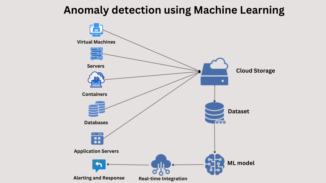
Figure 1: Log Anomaly Detection Using Machine Learning There are a number of techniques which attackers are using, the following are considered 'simple' measures which can be taken to evade IDS: Fragmentation: by sending fragmented packets, the attacker will be under the radar and can easily bypass the detection system's ability to detect the attack signature. Avoiding defaults: The TCP port utilised by a protocol does not always provide an indication to the protocol which is being transported. For example, an IDS may expect to detect a trojan on port 12345. If an attacker had reconfigured it to use a different port, the IDS may not be able to detect the presence of the trojan.
Coordinated, low-bandwidth attacks: coordinating a scan among numerous attackers (or agents) and allocating different ports or hosts to different attackers makes it difficult for the IDS to correlate the captured packets and deduce that a network scan is in progress. Address spoofing/proxying: attackers can increase the difficulty of the Security Administrators ability to determine the source of the attack by using poorly secured or incorrectly configured proxy servers to bounce an attack. If the source is spoofed and bounced by a server, it makes it very difficult for IDS to detect the origin of the attack. Pattern change evasion: IDS generally rely on 'pattern matching' to detect an attack. By changing the data used in the attack slightly, it may be possible to evade detection. For example, an Internet Message Access Protocol (IMAP) server may be vulnerable to a buffer overflow, and an IDS is able to detect the attack signature of 10 common attack tools. By modifying the payload sent by the tool, so that it does not resemble the data that the IDS expects, it may be possible to evade detection.
This article incorporates public domain material from Karen Scarfone, Peter Mell. Guide to Intrusion Detection and Prevention Systems, SP800-94 (PDF). National Institute of Standards and Technology. Retrieved 9 July 2025. A flow-based generative model is a generative model used in machine learning that explicitly models a probability distribution by leveraging normalizing flow, which is a statistical method using the change-of-variable law of probabilities to transform a simple distribution into a complex one. The direct modeling of likelihood provides many advantages. For example, the negative log-likelihood can be directly computed and minimized as the loss function. Additionally, novel samples can be generated by sampling from the initial distribution, and applying the flow transformation. In contrast, many alternative generative modeling methods, such as variational autoencoders (VAEs), generative adversarial networks (GANs), or diffusion models, do not explicitly represent the likelihood function.
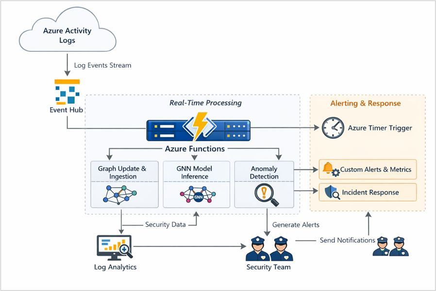
Figure 2: Graph Neural Networks for Azure Cloud Security Analytics: Anomaly ... Let z 0 {\displaystyle z_{0}} be a (possibly multivariate) random variable with distribution p 0 ( z 0 ) {\displaystyle p_{0}(z_{0})} . For i = 1 , . . . , K {\displaystyle i=1,...,K} , let z i = f i ( z i − 1 ) {\displaystyle z_{i}=f_{i}(z_{i-1})} be a sequence of random variables transformed from z 0 {\displaystyle z_{0}} . The functions f 1 , . . . , f K {\displaystyle f_{1},...,f_{K}} should be invertible, i.e. the inverse function f i − 1 {\displaystyle f_{i}^{-1}} exists. The final output z K {\displaystyle z_{K}} models the target distribution. The log likelihood of z K {\displaystyle z_{K}} is (see derivation): log I p K ( z K ) = log I p 0 ( z 0 ) − ∑ i = 1 K log I | det d f i ( z i − 1 ) d z i − 1 | {\displaystyle \log p_{K}(z_{K})=\log p_{0}(z_{0})-\sum _{i=1}^{K}\log \left|\det {\frac {df_{i}(z_{i-1})}{dz_{i-1}}}\right|} Learning probability distributions by differentiating such log Jacobians originated in the Infomax (maximum likelihood) approach to ICA, which forms a single-layer (K=1) flow-based model. Relatedly, the single layer precursor of conditional generative flows appeared in. To efficiently compute the log likelihood, the functions f 1 , . . . , f K {\displaystyle f_{1},...,f_{K}} should be easily invertible, and the determinants of their Jacobians should be simple to compute. In practice, the functions f 1 , . . . , f K {\displaystyle f_{1},...,f_{K}} are modeled using deep neural networks, and are trained to minimize the negative log-likelihood of data samples from the target distribution. These architectures are usually designed such that only the forward pass of the neural network is required in both the inverse and the Jacobian determinant calculations. Examples of such architectures include NICE, RealNVP, and Glow.
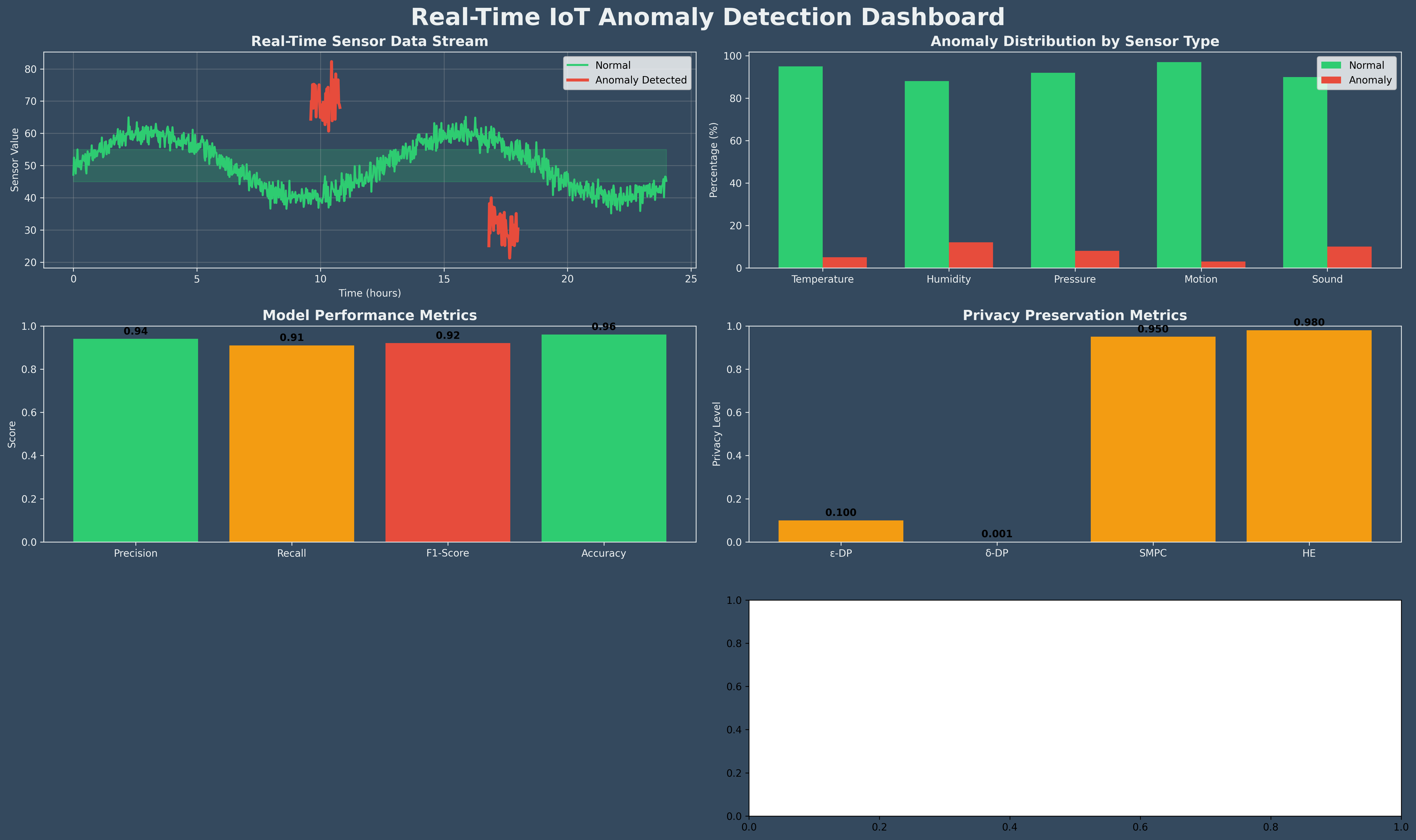
p 1 ( z 1 ) = p 0 ( z 0 ) | det d f 1 − 1 ( z 1 ) d z 1 | {\displaystyle p_{1}(z_{1})=p_{0}(z_{0})\left|\det {\frac {df_{1}^{-1}(z_{1})}{dz_{1}}}\right|} Figure 3: GitHub - vinitwadgaonkar/federated-learning-iot-anomaly-detection ... Where det d f 1 − 1 ( z 1 ) d z 1 {\displaystyle \det {\frac {df_{1}^{-1}(z_{1})}{dz_{1}}}} is the determinant of the Jacobian matrix of f 1 − 1 {\displaystyle f_{1}^{-1}} . By the inverse function theorem: p 1 ( z 1 ) = p 0 ( z 0 ) | det ( d f 1 ( z 0 ) d z 0 ) − 1 | {\displaystyle p_{1}(z_{1})=p_{0}(z_{0})\left|\det \left({\frac {df_{1}(z_{0})}{dz_{0}}}\right)^{-1}\right|} By the identity det ( A − 1 ) = det ( A ) − 1 {\displaystyle \det(A^{-1})=\det(A)^{-1}} (where A {\displaystyle A} is an invertible matrix), we have: p 1 ( z 1 ) = p 0 ( z 0 ) | det d f 1 ( z 0 ) d z 0 | − 1 {\displaystyle p_{1}(z_{1})=p_{0}(z_{0})\left|\det {\frac {df_{1}(z_{0})}{dz_{0}}}\right|^{-1}} log I p 1 ( z 1 ) = log I p 0 ( z 0 ) − log I | det d f 1 ( z 0 ) d z 0 | {\displaystyle \log p_{1}(z_{1})=\log p_{0}(z_{0})-\log \left|\det {\frac {df_{1}(z_{0})}{dz_{0}}}\right|} In general, the above applies to any z i {\displaystyle z_{i}} and z i − 1 {\displaystyle z_{i-1}} . Since log I p i ( z i ) {\displaystyle \log p_{i}(z_{i})} is equal to log I p i − 1 ( z i − 1 ) {\displaystyle \log p_{i-1}(z_{i-1})} subtracted by a non-recursive term, we can infer by induction that: log I p K ( z K ) = log I p 0 ( z 0 ) − ∑ i = 1 K log I | det d f i ( z i − 1 ) d z i − 1 | {\displaystyle \log p_{K}(z_{K})=\log p_{0}(z_{0})-\sum _{i=1}^{K}\log \left|\det {\frac {df_{i}(z_{i-1})}{dz_{i-1}}}\right|} D KL [ p ∗ ( x ) I p θ ( x ) ] = − E p ∗ ( x ) I [ log I p θ ( x ) ] + E p ∗ ( x ) I [ log I p ∗ ( x ) ] {\displaystyle D_{\text{KL}}[p^{*}(x)\|p_{\theta }(x)]=-\mathop {\mathbb {E} } _{p^{*}(x)}[\log p_{\theta }(x)]+\mathop {\mathbb {E} } _{p^{*}(x)}[\log p^{*}(x)]} The second term on the right-hand side of the equation corresponds to the entropy of the target distribution and is independent of the parameter θ {\displaystyle \theta } we want the model to learn, which only leaves the expectation of the negative log-likelihood to minimize under the target distribution. This intractable term can be approximated with a Monte-Carlo method by importance sampling. Indeed, if we have a dataset { x i } i = 1 N {\displaystyle \{x_{i}\}_{i=1}^{N}} of samples each independently drawn from the target distribution p ∗ ( x ) {\displaystyle p^{*}(x)} , then this term can be estimated as: − E ^ p ∗ ( x ) [ log I p θ ( x ) ] = − 1 N ∑ i = 0 N log I p θ ( x i ) {\displaystyle -{\hat {\mathop {\mathbb {E} } }}_{p^{*}(x)}[\log p_{\theta }(x)]=-{\frac {1}{N}}\sum _{i=0}^{N}\log p_{\theta }(x_{i})} 2. System Architecture & Core Working Principles a r g m i n θ D KL [ p ∗ ( x ) I p θ ( x ) ] {\displaystyle {\underset {\theta }{\operatorname {arg\,min} }}\ D_{\text{KL}}[p^{*}(x)\|p_{\theta }(x)]} a r g m a x θ ∑ i = 0 N log I p θ ( x i ) {\displaystyle {\underset {\theta }{\operatorname {arg\,max} }}\ \sum _{i=0}^{N}\log p_{\theta }(x_{i})} In other words, minimizing the Kullback–Leibler divergence between the model's likelihood and the target distribution is equivalent to maximizing the model likelihood under observed samples of the target distribution. A pseudocode for training normalizing flows is as follows: INPUT. dataset x 1 : n {\displaystyle x_{1:n}} , normalizing flow model f θ ( ⋅ ) , p 0 {\displaystyle f_{\theta }(\cdot ),p_{0}} .
SOLVE. max θ ∑ j log I p θ ( x j ) {\displaystyle \max _{\theta }\sum _{j}\log p_{\theta }(x_{j})} by gradient descent RETURN. θ ^ {\displaystyle {\hat {\theta }}} f θ − 1 {\displaystyle f_{\theta }^{-1}} is just z 1 = x 1 , z 2 = x 2 − m θ ( x 1 ) {\displaystyle z_{1}=x_{1},z_{2}=x_{2}-m_{\theta }(x_{1})} , and the Jacobian is just 1, that is, the flow is volume-preserving. When n = 1 {\displaystyle n=1} , this is seen as a curvy shearing along the x 2 {\displaystyle x_{2}} direction.
Its inverse is z 1 = x 1 , z 2 = e − s θ ( x 1 ) I ( x 2 − m θ ( x 1 ) ) {\displaystyle z_{1}=x_{1},z_{2}=e^{-s_{\theta }(x_{1})}\odot (x_{2}-m_{\theta }(x_{1}))} , and its Jacobian is ∏ i = 1 n e s θ ( z 1 , ) {\displaystyle \prod _{i=1}^{n}e^{s_{\theta }(z_{1,})}} . The NICE model is recovered by setting s θ = 0 {\displaystyle s_{\theta }=0} . Since the Real NVP map keeps the first and second halves of the vector x {\displaystyle x} separate, it's usually required to add a permutation ( x 1 , x 2 ) I ( x 2 , x 1 ) {\displaystyle (x_{1},x_{2})\mapsto (x_{2},x_{1})} after every Real NVP layer.
channel-wise affine transform y c i j = s c ( x c i j + b c ) {\displaystyle y_{cij}=s_{c}(x_{cij}+b_{c})} with Jacobian ∏ c s c H W {\displaystyle \prod _{c}s_{c}^{HW}} . invertible 1x1 convolution z c i j = ∑ c ′ K c c ′ y c i j {\displaystyle z_{cij}=\sum _{c'}K_{cc'}y_{cij}} with Jacobian det ( K ) H W {\displaystyle \det(K)^{HW}} . Here K {\displaystyle K} is any invertible matrix. Real NVP, with Jacobian as described in Real NVP. The idea of using the invertible 1x1 convolution is to permute all layers in general, instead of merely permuting the first and second half, as in Real NVP.
x 1 ∼ N ( µ 1 , σ 1 2 ) x 2 ∼ N ( µ 2 ( x 1 ) , σ 2 ( x 1 ) 2 ) I x n ∼ N ( µ n ( x 1 : n − 1 ) , σ n ( x 1 : n − 1 ) 2 ) {\displaystyle {\begin{aligned}x_{1}\sim &N(\mu _{1},\sigma _{1}^{2})\\x_{2}\sim &N(\mu _{2}(x_{1}),\sigma _{2}(x_{1})^{2})\\&\cdots \\x_{n}\sim &N(\mu _{n}(x_{1:n-1}),\sigma _{n}(x_{1:n-1})^{2})\\\end{aligned}}} where µ i : R i − 1 → R {\displaystyle \mu _{i}:\mathbb {R} ^{i-1}\to \mathbb {R} } and σ i : R i − 1 → ( 0 , ∞ ) {\displaystyle \sigma _{i}:\mathbb {R} ^{i-1}\to (0,\infty )} are fixed functions that define the autoregressive model. By the reparameterization trick, the autoregressive model is generalized to a normalizing flow: x 1 = µ 1 + σ 1 z 1 x 2 = µ 2 ( x 1 ) + σ 2 ( x 1 ) z 2 I x n = µ n ( x 1 : n − 1 ) + σ n ( x 1 : n − 1 ) z n {\displaystyle {\begin{aligned}x_{1}=&\mu _{1}+\sigma _{1}z_{1}\\x_{2}=&\mu _{2}(x_{1})+\sigma _{2}(x_{1})z_{2}\\&\cdots \\x_{n}=&\mu _{n}(x_{1:n-1})+\sigma _{n}(x_{1:n-1})z_{n}\\\end{aligned}}} The autoregressive model is recovered by setting z ∼ N ( 0 , I n ) {\displaystyle z\sim N(0,I_{n})} . The forward mapping is slow (because it's sequential), but the backward mapping is fast (because it's parallel). The Jacobian matrix is lower-diagonal, so the Jacobian is σ 1 σ 2 ( x 1 ) I σ n ( x 1 : n − 1 ) {\displaystyle \sigma _{1}\sigma _{2}(x_{1})\cdots \sigma _{n}(x_{1:n-1})} . Reversing the two maps f θ {\displaystyle f_{\theta }} and f θ − 1 {\displaystyle f_{\theta }^{-1}} of MAF results in Inverse Autoregressive Flow (IAF), which has fast forward mapping and slow backward mapping.
x = F ( z 0 ) = z T = z 0 + ∫ 0 T f ( z t , t ) d t {\displaystyle x=F(z_{0})=z_{T}=z_{0}+\int _{0}^{T}f(z_{t},t)dt} where f {\displaystyle f} is an arbitrary function and can be modeled with e.g. neural networks. The inverse function is then naturally: z 0 = F − 1 ( x ) = z T + ∫ T 0 f ( z t , t ) d t = z T − ∫ 0 T f ( z t , t ) d t {\displaystyle z_{0}=F^{-1}(x)=z_{T}+\int _{T}^{0}f(z_{t},t)dt=z_{T}-\int _{0}^{T}f(z_{t},t)dt} And the log-likelihood of x {\displaystyle x} can be found as: log I ( p ( x ) ) = log I ( p ( z 0 ) ) − ∫ 0 T Tr [ ∂ f ∂ z t ] d t {\displaystyle \log(p(x))=\log(p(z_{0}))-\int _{0}^{T}{\text{Tr}}\left[{\frac {\partial f}{\partial z_{t}}}\right]dt} Since the trace depends only on the diagonal of the Jacobian ∂ z t f {\displaystyle \partial _{z_{t}}f} , this allows "free-form" Jacobian. Here, "free-form" means that there is no restriction on the Jacobian's form. It is contrasted with previous discrete models of normalizing flow, where the Jacobian is carefully designed to be only upper- or lower-diagonal, so that the Jacobian can be evaluated efficiently.
The trace can be estimated by "Hutchinson's trick":Given any matrix W ∈ R n × n {\displaystyle W\in \mathbb {R} ^{n\times n}} , and any random u ∈ R n {\displaystyle u\in \mathbb {R} ^{n}} with E [ u u T ] = I {\displaystyle E[uu^{T}]=I} , we have E [ u T W u ] = t r ( W ) {\displaystyle E[u^{T}Wu]=tr(W)} . (Proof: expand the expectation directly.)Usually, the random vector is sampled from N ( 0 , I ) {\displaystyle N(0,I)} (normal distribution) or { ± n − 1 / 2 } n {\displaystyle \{\pm n^{-1/2}\}^{n}} (Rademacher distribution). When f {\displaystyle f} is implemented as a neural network, neural ODE methods would be needed. Indeed, CNF was first proposed in the same paper that proposed neural ODE. There are two main deficiencies of CNF, one is that a continuous flow must be a homeomorphism, thus preserve orientation and ambient isotopy (for example, it's impossible to flip a left-hand to a right-hand by continuous deforming of space, and it's impossible to turn a sphere inside out, or undo a knot), and the other is that the learned flow f {\displaystyle f} might be ill-behaved, due to degeneracy (that is, there are an infinite number of possible f {\displaystyle f} that all solve the same problem). By adding extra dimensions, the CNF gains enough freedom to reverse orientation and go beyond ambient isotopy (just like how one can pick up a polygon from a desk and flip it around in 3-space, or unknot a knot in 4-space), yielding the "augmented neural ODE". Any homeomorphism of R n {\displaystyle \mathbb {R} ^{n}} can be approximated by a neural ODE operating on R 2 n + 1 {\displaystyle \mathbb {R} ^{2n+1}} , proved by combining Whitney embedding theorem for manifolds and the universal approximation theorem for neural networks. To regularize the flow f {\displaystyle f} , one can impose regularization losses. The paper proposed the following regularization loss based on optimal transport theory: λ K ∫ 0 T I f ( z t , t ) I 2 d t + λ J ∫ 0 T I ∇ z f ( z t , t ) I F 2 d t {\displaystyle \lambda _{K}\int _{0}^{T}\left\|f(z_{t},t)\right\|^{2}dt+\lambda _{J}\int _{0}^{T}\left\|\nabla _{z}f(z_{t},t)\right\|_{F}^{2}dt} where λ K , λ J > 0 {\displaystyle \lambda _{K},\lambda _{J}>0} are hyperparameters. The first term punishes the model for oscillating the flow field over time, and the second term punishes it for oscillating the flow field over space. Both terms together guide the model into a flow that is smooth (not "bumpy") over space and time.
The unit hypersphere: S n − 1 = { x ∈ R n : x ′ x = 1 } {\displaystyle \mathbb {S} ^{n-1}=\{\mathbf {x} \in \mathbb {R} ^{n}:\mathbf {x} '\mathbf {x} =1\}} , where flows can be used to generalize e.g. Von Mises-Fisher or uniform spherical distributions. The simplex interior: ∆ n − 1 = { p = ( p 1 , … , p n ) ∈ R n : p i > 0 , ∑ i p i = 1 } {\displaystyle \Delta ^{n-1}=\{\mathbf {p} =(p_{1},\dots ,p_{n})\in \mathbb {R} ^{n}:p_{i}>0,\sum _{i}p_{i}=1\}} , where n {\displaystyle n} -way categorical distributions live; and where flows can be used to generalize e.g. Dirichlet, or uniform simplex distributions. As a first example of a spherical manifold flow transform, consider the normalized linear transform, which radially projects onto the unit sphere the output of an invertible linear transform, parametrized by the n -by- n {\displaystyle n{\text{-by-}}n} invertible matrix M {\displaystyle \mathbf {M} } : f lin ( x ; M ) = M x I M x I {\displaystyle f_{\text{lin}}(\mathbf {x} ;\mathbf {M} )={\frac {\mathbf {Mx} }{\lVert \mathbf {Mx} \rVert }}} In full Euclidean space, f lin : R n → R n {\displaystyle f_{\text{lin}}:\mathbb {R} ^{n}\to \mathbb {R} ^{n}} is not invertible, but if we restrict the domain and co-domain to the unit sphere, then f lin : S n − 1 → S n − 1 {\displaystyle f_{\text{lin}}:\mathbb {S} ^{n-1}\to \mathbb {S} ^{n-1}} is invertible (more specifically it is a bijection and a homeomorphism and a diffeomorphism), with inverse f lin ( ⋅ ; M − 1 ) {\displaystyle f_{\text{lin}}(\cdot \,;\mathbf {M} ^{-1})} . The Jacobian of f lin : R n → R n {\displaystyle f_{\text{lin}}:\mathbb {R} ^{n}\to \mathbb {R} ^{n}} , at y = f lin ( x ; M ) {\displaystyle \mathbf {y} =f_{\text{lin}}(\mathbf {x} ;\mathbf {M} )} is I M x I − 1 ( I n − y y ′ ) M {\displaystyle \lVert \mathbf {Mx} \rVert ^{-1}(\mathbf {I} _{n}-\mathbf {yy} ')\mathbf {M} } , which has rank n − 1 {\displaystyle n-1} and determinant of zero; while as explained here, the factor (see subsection below) relating source and transformed densities is: I M x I − n | det I M | {\displaystyle \lVert \mathbf {Mx} \rVert ^{-n}\left|\operatorname {det} \mathbf {M} \right|} .
P X ( x ) volume I ( U ) ≈ P Y ( y ) volume I ( V ) {\displaystyle P_{X}(\mathbf {x} )\operatorname {volume} (U)\approx P_{Y}(\mathbf {y} )\operatorname {volume} (V)} where volume (for very small regions) is given by Lebesgue measure in m {\displaystyle m} -dimensional tangent space. By making the regions infinitessimally small, the factor relating the two densities is the ratio of volumes, which we term the differential volume ratio. To obtain concrete formulas for volume on the m {\displaystyle m} -dimensional manifold, we construct U {\displaystyle U} by mapping an m {\displaystyle m} -dimensional rectangle in (local) coordinate space to the manifold via a smooth embedding function: R m → R n {\displaystyle \mathbb {R} ^{m}\to \mathbb {R} ^{n}} . At very small scale, the embedding function becomes essentially linear so that U {\displaystyle U} is a parallelotope (multidimensional generalization of a parallelogram). Similarly, the flow transform, f {\displaystyle f} becomes linear, so that the image, V = f ( U ) {\displaystyle V=f(U)} is also a parallelotope. In R m {\displaystyle \mathbb {R} ^{m}} , we can represent an m {\displaystyle m} -dimensional parallelotope with an m -by- m {\displaystyle m{\text{-by-}}m} matrix whose column-vectors are a set of edges (meeting at a common vertex) that span the paralellotope. The volume is given by the absolute value of the determinant of this matrix. If more generally (as is the case here), an m {\displaystyle m} -dimensional paralellotope is embedded in R n {\displaystyle \mathbb {R} ^{n}} , it can be represented with a (tall) n -by- m {\displaystyle n{\text{-by-}}m} matrix, say V {\displaystyle \mathbf {V} } . Denoting the parallelotope as / V / {\displaystyle /\mathbf {V} \!/} , its volume is then given by the square root of the Gram determinant: volume I / V / = | det I ( V ′ V ) | {\displaystyle \operatorname {volume} /\mathbf {V} \!/={\sqrt {\left|\operatorname {det} (\mathbf {V} '\mathbf {V} )\right|}}} In the sections below, we show various ways to use this volume formula to derive the differential volume ratio.
3. Software Implementation, Frameworks & Protocols e : p ~ = ( p 1 … , p n − 1 ) I p = ( p 1 … , p n − 1 , 1 − ∑ i = 1 n − 1 p i ) {\displaystyle e:{\tilde {\mathbf {p} }}=(p_{1}\dots ,p_{n-1})\mapsto \mathbf {p} =(p_{1}\dots ,p_{n-1},1-\sum _{i=1}^{n-1}p_{i})} which maps a conveniently chosen, ( n − 1 ) {\displaystyle (n-1)} -dimensional representation, p ~ {\displaystyle {\tilde {\mathbf {p} }}} , to the embedded manifold. The n -by- ( n − 1 ) {\displaystyle n{\text{-by-}}(n-1)} Jacobian is E = [ I n − 1 − 1 ′ ] {\displaystyle \mathbf {E} ={\begin{bmatrix}\mathbf {I} _{n-1}\\-{\boldsymbol {1}}'\end{bmatrix}}} . To define U {\displaystyle U} , the differential volume element at the transformation input ( p ∈ ∆ n − 1 {\displaystyle \mathbf {p} \in \Delta ^{n-1}} ), we start with a rectangle in p ~ {\displaystyle {\tilde {\mathbf {p} }}} -space, having (signed) differential side-lengths, d p 1 , … , d p n − 1 {\displaystyle dp_{1},\dots ,dp_{n-1}} from which we form the square diagonal matrix D {\displaystyle \mathbf {D} } , the columns of which span the rectangle. At very small scale, we get U = e ( D ) = / E D / {\displaystyle U=e(\mathbf {D} )=/\mathbf {ED} \!/} , with: volume I ( U ) = | det I ( D E ′ E D ) | = | det I ( E ′ E ) | | det I D ) | = n ∏ i = 1 n − 1 | d p i | {\displaystyle \operatorname {volume} (U)={\sqrt {\left|\operatorname {det} (\mathbf {DE} '\mathbf {ED} )\right|}}={\sqrt {\left|\operatorname {det} (\mathbf {E} '\mathbf {E} )\right|}}\,\left|\operatorname {det} \mathbf {D} )\right|={\sqrt {n}}\prod _{i=1}^{n-1}\left|dp_{i}\right|} To understand the geometric interpretation of the factor n {\displaystyle {\sqrt {n}}} , see the example for the 1-simplex in the diagram at right. The differential volume element at the transformation output ( q ∈ ∆ n − 1 {\displaystyle \mathbf {q} \in \Delta ^{n-1}} ), is the parallelotope, V = f ( U ) = / F p E D / {\displaystyle V=f(U)=/\mathbf {F_{p}ED} \!/} , where F p {\displaystyle \mathbf {F_{p}} } is the n -by- n {\displaystyle n{\text{-by-}}n} Jacobian of f {\displaystyle f} at p = e ( p ~ ) {\displaystyle \mathbf {p} =e({\tilde {\mathbf {p} }})} . Its volume is: volume I ( V ) = | det I ( D E ′ F p ′ F p E D ) | = | det I ( E ′ F p ′ F p E ) | | det I D ) | {\displaystyle \operatorname {volume} (V)={\sqrt {\left|\operatorname {det} (\mathbf {DE} '\mathbf {F_{p}} '\mathbf {F_{p}ED} )\right|}}={\sqrt {\left|\operatorname {det} (\mathbf {E} '\mathbf {F_{p}} '\mathbf {F_{p}E} )\right|}}\,\left|\operatorname {det} \mathbf {D} )\right|} so that the factor | det I D ) | {\displaystyle \left|\operatorname {det} \mathbf {D} )\right|} cancels in the volume ratio, which can now already be numerically evaluated. It can however be rewritten in a sometimes more convenient form by also introducing the representation function, r : p I p ~ {\displaystyle r:\mathbf {p} \mapsto {\tilde {\mathbf {p} }}} , which simply extracts the first ( n − 1 ) {\displaystyle (n-1)} components. The Jacobian is R = [ I n 0 ] {\displaystyle \mathbf {R} ={\begin{bmatrix}\mathbf {I} _{n}&{\boldsymbol {0}}\end{bmatrix}}} . Observe that, since e I r I f = f {\displaystyle e\circ r\circ f=f} , the chain rule for function composition gives: E R F p = F p {\displaystyle \mathbf {ERF_{p}} =\mathbf {F_{p}} } . By plugging this expansion into the above Gram determinant and then refactoring it as a product of determinants of square matrices, we can extract the factor | det I ( E ′ E ) | = n {\displaystyle {\sqrt {\left|\operatorname {det} (\mathbf {E} '\mathbf {E} )\right|}}={\sqrt {n}}} , which now also cancels in the ratio, which finally simpifies to the determinant of the Jacobian of the "sandwiched" flow transformation, r I f I e {\displaystyle r\circ f\circ e} : R f ∆ ( p ) = volume I ( V ) volume I ( U ) = | det I ( R F p E ) | {\displaystyle R_{f}^{\Delta }(\mathbf {p} )={\frac {\operatorname {volume} (V)}{\operatorname {volume} (U)}}=\left|\operatorname {det} (\mathbf {RF_{p}E} )\right|} which, if p ∼ P P {\displaystyle \mathbf {p} \sim P_{\mathbf {P} }} , can be used to derive the pushforward density after a change of variables, q = f ( p ) {\displaystyle \mathbf {q} =f(\mathbf {p} )} : P Q ( q ) = P P ( p ) R f ∆ ( p ) , where p = f − 1 ( q ) {\displaystyle P_{\mathbf {Q} }(\mathbf {q} )={\frac {P_{\mathbf {P} }(\mathbf {p} )}{R_{f}^{\Delta }(\mathbf {p} )}}\,,\;{\text{where}}\;\;\mathbf {p} =f^{-1}(\mathbf {q} )} This formula is valid only because the simplex is flat and the Jacobian, E {\displaystyle \mathbf {E} } is constant. The more general case for curved manifolds is discussed below, after we present two concrete examples of simplex flow transforms.
q = f cal ( p ; a , c ) = softmax I ( a − 1 log I p + c ) I p = f cal − 1 ( q ; a , c ) = softmax I ( a log I q − a c ) {\displaystyle \mathbf {q} =f_{\text{cal}}(\mathbf {p} ;a,\mathbf {c} )=\operatorname {softmax} (a^{-1}\log \mathbf {p} +\mathbf {c} )\;\iff \;\mathbf {p} =f_{\text{cal}}^{-1}(\mathbf {q} ;a,\mathbf {c} )=\operatorname {softmax} (a\log \mathbf {q} -a\mathbf {c} )} where the log is applied elementwise. After some algebra the differential volume ratio can be expressed as: R cal ∆ ( p ; a , c ) = | det I ( R F p E ) | = | a | 1 − n ∏ i = 1 n q i p i {\displaystyle R_{\text{cal}}^{\Delta }(\mathbf {p} ;a,\mathbf {c} )=\left|\operatorname {det} (\mathbf {RF_{p}E} )\right|=\left|a\right|^{1-n}\prod _{i=1}^{n}{\frac {q_{i}}{p_{i}}}} This result can also be obtained by factoring the density of the SGB distribution, which is obtained by sending Dirichlet variates through f cal {\displaystyle f_{\text{cal}}} . While calibration transforms are most often trained as discriminative models, the reinterpretation here as a probabilistic flow allows also the design of generative calibration models based on this transform. When used for calibration, the restriction a > 0 {\displaystyle a>0} can be imposed to prevent direction reversal in log-probability space. With the additional restriction c = 0 {\displaystyle \mathbf {c} ={\boldsymbol {0}}} , this transform (with discriminative training) is known in machine learning as temperature scaling.
q = f gcal ( p ; A , c ) = softmax I ( A log I p + c ) , subject to A 1 = λ 1 {\displaystyle \mathbf {q} =f_{\text{gcal}}(\mathbf {p} ;\mathbf {A} ,\mathbf {c} )=\operatorname {softmax} (\mathbf {A} \log \mathbf {p} +\mathbf {c} )\,,\;{\text{subject to}}\;\mathbf {A1} =\lambda \mathbf {1} } where the condition that A {\displaystyle \mathbf {A} } has 1 {\displaystyle \mathbf {1} } as an eigenvector ensures invertibility by sidestepping the information loss due to the invariance: softmax I ( x + α 1 ) = softmax I ( x ) {\displaystyle \operatorname {softmax} (\mathbf {x} +\alpha \mathbf {1} )=\operatorname {softmax} (\mathbf {x} )} . Note in particular that A = λ I n {\displaystyle \mathbf {A} =\lambda \mathbf {I} _{n}} is the only allowed diagonal parametrization, in which case we recover f cal ( p ; λ − 1 , c ) {\displaystyle f_{\text{cal}}(\mathbf {p} ;\lambda ^{-1},\mathbf {c} )} , while (for n > 2 {\displaystyle n>2} ) generalization is possible with non-diagonal matrices. The inverse is: p = f gcal − 1 ( q ; A , c ) = f gcal ( q ; A − 1 , − A − 1 c ) , where A 1 = λ 1 I A − 1 1 = λ − 1 1 {\displaystyle \mathbf {p} =f_{\text{gcal}}^{-1}(\mathbf {q} ;\mathbf {A} ,\mathbf {c} )=f_{\text{gcal}}(\mathbf {q} ;\mathbf {A} ^{-1},-\mathbf {A} ^{-1}\mathbf {c} )\,,\;{\text{where}}\;\mathbf {A1} =\lambda \mathbf {1} \Longrightarrow \mathbf {A} ^{-1}\mathbf {1} =\lambda ^{-1}\mathbf {1} } R gcal ∆ ( p ; A , c ) = | det I ( A ) | | λ | ∏ i = 1 n q i p i {\displaystyle R_{\text{gcal}}^{\Delta }(\mathbf {p} ;\mathbf {A} ,\mathbf {c} )={\frac {\left|\operatorname {det} (\mathbf {A} )\right|}{|\lambda |}}\prod _{i=1}^{n}{\frac {q_{i}}{p_{i}}}} If f gcal {\displaystyle f_{\text{gcal}}} is to be used as a calibration transform, further constraint could be imposed, for example that A {\displaystyle \mathbf {A} } be positive definite, so that ( A x ) ′ x > 0 {\displaystyle (\mathbf {Ax} )'\mathbf {x} >0} , which avoids direction reversals. (This is one possible generalization of a > 0 {\displaystyle a>0} in the f cal {\displaystyle f_{\text{cal}}} parameter.) For n = 2 {\displaystyle n=2} , a > 0 {\displaystyle a>0} and A {\displaystyle \mathbf {A} } positive definite, then f cal {\displaystyle f_{\text{cal}}} and f gcal {\displaystyle f_{\text{gcal}}} are equivalent in the sense that in both cases, log I p 1 p 2 I log I q 1 q 2 {\displaystyle \log {\frac {p_{1}}{p_{2}}}\mapsto \log {\frac {q_{1}}{q_{2}}}} is a straight line, the (positive) slope and offset of which are functions of the transform parameters. For n > 2 , {\displaystyle n>2,} f gcal {\displaystyle f_{\text{gcal}}} does generalize f cal {\displaystyle f_{\text{cal}}} . It must however be noted that chaining multiple f gcal {\displaystyle f_{\text{gcal}}} flow transformations does not give a further generalization, because: f gcal ( ⋅ ; A 1 , c 1 ) I f gcal ( ⋅ ; A 2 , c 2 ) = f gcal ( ⋅ ; A 1 A 2 , c 1 + A 1 c 2 ) {\displaystyle f_{\text{gcal}}(\cdot \,;\mathbf {A} _{1},\mathbf {c} _{1})\circ f_{\text{gcal}}(\cdot \,;\mathbf {A} _{2},\mathbf {c} _{2})=f_{\text{gcal}}(\cdot \,;\mathbf {A} _{1}\mathbf {A} _{2},\mathbf {c} _{1}+\mathbf {A} _{1}\mathbf {c} _{2})} In fact, the set of f gcal {\displaystyle f_{\text{gcal}}} transformations form a group under function composition. The set of f cal {\displaystyle f_{\text{cal}}} transformations form a subgroup. Also see: Dirichlet calibration, which generalizes f gcal {\displaystyle f_{\text{gcal}}} , by not placing any restriction on the matrix, A {\displaystyle \mathbf {A} } , so that invertibility is not guaranteed. While Dirichlet calibration is trained as a discriminative model, f gcal {\displaystyle f_{\text{gcal}}} can also be trained as part of a generative calibration model.
4. Practical Deployment, Analysis & Case Studies R f ( x ) = | det I ( R y F x E x ) | | det I ( E y ′ E y ) | | det I ( E x ′ E x ) | {\displaystyle R_{f}(\mathbf {x} )=\left|\operatorname {det} (\mathbf {R_{y}F_{x}E_{x}} )\right|\,{\frac {\sqrt {\left|\operatorname {det} (\mathbf {E} _{\mathbf {y} }'\mathbf {E_{y}} )\right|}}{\sqrt {\left|\operatorname {det} (\mathbf {E} _{\mathbf {x} }'\mathbf {E_{x}} )\right|}}}} For geometric insight, consider S 2 {\displaystyle \mathbf {S} ^{2}} , where the spherical coordinates are co-latitude, θ ∈ [ 0 , π ] {\displaystyle \theta \in [0,\pi ]} and longitude, ϕ ∈ [ 0 , 2 π ) {\displaystyle \phi \in [0,2\pi )} . At x = e ( θ , ϕ ) {\displaystyle \mathbf {x} =e(\theta ,\phi )} , we get | det I ( E x ′ E x ) | = sin I θ {\displaystyle {\sqrt {\left|\operatorname {det} (\mathbf {E} _{\mathbf {x} }'\mathbf {E_{x}} )\right|}}=\sin \theta } , which gives the radius of the circle at that latitude (compare e.g. polar circle to equator). The differential volume (surface area on the sphere) is: sin I θ d θ d ϕ {\displaystyle \sin \theta \,d\theta \,d\phi } . The above derivation for R f {\displaystyle R_{f}} is fragile in the sense that when using fixed functions e , r {\displaystyle e,r} , there may be places where they are not well-defined, for example at the poles of the 2-sphere where longitude is arbitrary. This problem is sidestepped (using standard manifold machinery) by generalizing to local coordinates (charts), where in the vicinities of x , y ∈ M {\displaystyle \mathbf {x} ,\mathbf {y} \in {\mathcal {M}}} , we map from local m {\displaystyle m} -dimensional coordinates to R n {\displaystyle \mathbb {R} ^{n}} and back using the respective function pairs e x , r x {\displaystyle e_{\mathbf {x} },r_{\mathbf {x} }} and e y , r y {\displaystyle e_{\mathbf {y} },r_{\mathbf {y} }} . We continue to use the same notation for the Jacobians of these functions ( E x , E y , R y {\displaystyle \mathbf {E_{x}} ,\mathbf {E_{y}} ,\mathbf {R_{y}} } ), so that the above formula for R f {\displaystyle R_{f}} remains valid. We can however, choose our local coordinate system in a way that simplifies the expression for R f {\displaystyle R_{f}} and indeed also its practical implementation. Let π : P → R n {\displaystyle \pi :{\mathcal {P}}\to \mathbb {R} ^{n}} be a smooth idempotent projection ( π I π = π {\displaystyle \pi \circ \pi =\pi } ) from the projectible set, P ⊆ R n {\displaystyle {\mathcal {P}}\subseteq \mathbb {R} ^{n}} , onto the embedded manifold. For example: The positive orthant of R n {\displaystyle \mathbb {R} ^{n}} is projected onto the simplex as: π ( z ) = ( ∑ i = 1 n z i ) − 1 z {\displaystyle \pi (\mathbf {z} )={\bigl (}\sum _{i=1}^{n}z_{i}{\bigr )}^{-1}\mathbf {z} } Non-zero vectors in R n {\displaystyle \mathbb {R} ^{n}} are projected onto the unit sphere as: π ( z ) = ( ∑ i = 1 n z i 2 ) − 1 2 z {\displaystyle \pi (\mathbf {z} )={\bigl (}\sum _{i=1}^{n}z_{i}^{2}{\bigr )}^{-{\frac {1}{2}}}\mathbf {z} } For every x ∈ M {\displaystyle \mathbf {x} \in {\mathcal {M}}} , we require of π {\displaystyle \pi } that its n -by- n {\displaystyle n{\text{-by-}}n} Jacobian, Π x {\displaystyle {\boldsymbol {\Pi _{x}}}} has rank m {\displaystyle m} (the manifold dimension), in which case Π x {\displaystyle {\boldsymbol {\Pi _{x}}}} is an idempotent linear projection onto the local tangent space (orthogonal for the unit sphere: I n − x x ′ {\displaystyle \mathbf {I} _{n}-\mathbf {xx} '} ; oblique for the simplex: I n − x 1 ′ {\displaystyle \mathbf {I} _{n}-{\boldsymbol {x1}}'} ). The columns of Π x {\displaystyle {\boldsymbol {\Pi _{x}}}} span the m {\displaystyle m} -dimensional tangent space at x {\displaystyle \mathbf {x} } . We use the notation, T x {\displaystyle \mathbf {T_{x}} } for any n -by- m {\displaystyle n{\text{-by-}}m} matrix with orthonormal columns ( T x ′ T x = I m {\displaystyle \mathbf {T} _{\mathbf {x} }'\mathbf {T_{x}} =\mathbf {I} _{m}} ) that span the local tangent space. Also note: Π x T x = T x {\displaystyle {\boldsymbol {\Pi _{x}}}\mathbf {T_{x}} =\mathbf {T_{x}} } . We can now choose our local coordinate embedding function, e x : R m → R n {\displaystyle e_{\mathbf {x} }:\mathbb {R} ^{m}\to \mathbb {R} ^{n}} : e x ( x ~ ) = π ( x + T x x ~ ) , with Jacobian: E x = T x at x ~ = 0 . {\displaystyle e_{\mathbf {x} }({\tilde {x}})=\pi (\mathbf {x} +\mathbf {T_{x}{\tilde {x}}} )\,,{\text{with Jacobian:}}\,\mathbf {E_{x}} =\mathbf {T_{x}} \,{\text{at}}\,{\tilde {\mathbf {x} }}=\mathbf {0} .} Since the Jacobian is injective (full rank: m {\displaystyle m} ), a local (not necessarily unique) left inverse, say r x ∗ {\displaystyle r_{\mathbf {x} }^{*}} with Jacobian R x ∗ {\displaystyle \mathbf {R} _{\mathbf {x} }^{*}} , exists such that r x ∗ ( e x ( x ~ ) ) = x ~ {\displaystyle r_{\mathbf {x} }^{*}(e_{\mathbf {x} }({\tilde {x}}))={\tilde {x}}} and R x ∗ T x = I m {\displaystyle \mathbf {R} _{\mathbf {x} }^{*}\mathbf {T_{x}} =\mathbf {I} _{m}} . In practice we do not need the left inverse function itself, but we do need its Jacobian, for which the above equation does not give a unique solution. We can however enforce a unique solution for the Jacobian by choosing the left inverse as, r x : R n → R m {\displaystyle r_{\mathbf {x} }:\mathbb {R} ^{n}\to \mathbb {R} ^{m}} : r x ( z ) = r x ∗ ( π ( z ) ) , with Jacobian: R x = T x ′ {\displaystyle r_{\mathbf {x} }(\mathbf {z} )=r_{\mathbf {x} }^{*}(\pi (\mathbf {z} ))\,,{\text{with Jacobian:}}\,\mathbf {R_{x}} =\mathbf {T} _{\mathbf {x} }'} We can now finally plug E x = T x {\displaystyle \mathbf {E_{x}} =\mathbf {T_{x}} } and R y = T y ′ {\displaystyle \mathbf {R_{y}} =\mathbf {T} _{\mathbf {y} }'} into our previous expression for R f {\displaystyle R_{f}} , the differential volume ratio, which because of the orthonormal Jacobians, simplifies to: R f ( x ) = | det I ( T y ′ F x T x ) | {\displaystyle R_{f}(\mathbf {x} )=\left|\operatorname {det} (\mathbf {T_{y}} '\mathbf {F_{x}T_{x}} )\right|} Sorrenson et al.(2023) give a solution for computationally efficient stochastic parameter gradient approximation for log I R f .
{\displaystyle \log R_{f}.} For some hand-designed flow transforms, R f {\displaystyle R_{f}} can be analytically derived in closed form, for example the above-mentioned simplex calibration transforms. Further examples are given below in the section on simple spherical flows. On a software platform equipped with linear algebra and automatic differentiation, R f ( x ) = | det I ( T y ′ F x T x ) | {\displaystyle R_{f}(\mathbf {x} )=\left|\operatorname {det} (\mathbf {T_{y}} '\mathbf {F_{x}T_{x}} )\right|} can be automatically evaluated, given access to only x , f , π {\displaystyle \mathbf {x} ,f,\pi } . But this is expensive for high-dimensional data, with at least O ( n 3 ) {\displaystyle {\mathcal {O}}(n^{3})} computational costs. Even then, the slow automatic solution can be invaluable as a tool for numerically verifying hand-designed closed-form solutions.
To derive the inverse transform, with suitable restrictions on the parameters to ensure invertibility. To derive in simple closed form the differential volume ratio, R f {\displaystyle R_{f}} . An interesting property of these simple spherical flows is that they don't make use of any non-linearities apart from the radial projection. Even the simplest of them, the normalized translation flow, can be chained to form perhaps surprisingly flexible distributions.
y = f trans ( x ; c ) = x + c I x + c I , where I c I < 1 {\displaystyle \mathbf {y} =f_{\text{trans}}(\mathbf {x} ;\mathbf {c} )={\frac {\mathbf {x} +\mathbf {c} }{\lVert \mathbf {x} +\mathbf {c} \rVert }}\,,\;{\text{where}}\;\lVert \mathbf {c} \rVert <1} The inverse function may be derived by considering, for I > 0 {\displaystyle \ell >0} : y = I − 1 ( x + c ) {\displaystyle \mathbf {y} =\ell ^{-1}(\mathbf {x} +\mathbf {c} )} and then using x ′ x = 1 {\displaystyle \mathbf {x} '\mathbf {x} =1} to get a quadratic equation to recover I {\displaystyle \ell } , which gives: x = f trans − 1 ( y ; c ) = I y − c , where I = y ′ c + ( y ′ c ) 2 + 1 − c ′ c {\displaystyle \mathbf {x} =f_{\text{trans}}^{-1}(\mathbf {y} ;\mathbf {c} )=\ell \mathbf {y} -\mathbf {c} \,,{\text{where}}\;\ell =\mathbf {y} '\mathbf {c} +{\sqrt {(\mathbf {y} '\mathbf {c} )^{2}+1-\mathbf {c} '\mathbf {c} }}} from which we see that we need I c I < 1 {\displaystyle \lVert \mathbf {c} \rVert <1} to keep I {\displaystyle \ell } real and positive for all y ∈ S n − 1 {\displaystyle \mathbf {y} \in \mathbb {S} ^{n-1}} . The differential volume ratio is given (without derivation) by Boulerice & Ducharme(1994) as: R trans ( x ; c ) = 1 + x ′ c I x + c I n {\displaystyle R_{\text{trans}}(\mathbf {x} ;\mathbf {c} )={\frac {1+\mathbf {x} '\mathbf {c} }{\lVert \mathbf {x} +\mathbf {c} \rVert ^{n}}}} By a laborious manipulation of R f ( x ) = | det I ( T y ′ F x T x ) | {\displaystyle R_{f}(\mathbf {x} )=\left|\operatorname {det} (\mathbf {T_{y}} '\mathbf {F_{x}T_{x}} )\right|} . By setting M = I n {\displaystyle \mathbf {M} =\mathbf {I} _{n}} in R aff ( x ; M , c ) {\displaystyle R_{\text{aff}}(\mathbf {x} ;\mathbf {M} ,\mathbf {c} )} , which is given below. Finally, it is worth noting that f trans {\displaystyle f_{\text{trans}}} and f trans − 1 {\displaystyle f_{\text{trans}}^{-1}} do not have the same functional form.
y = f lin ( x ; M ) = M x I M x I I x = f lin − 1 ( y ; M ) = f lin ( y ; M − 1 ) = M − 1 y I M − 1 y I {\displaystyle \mathbf {y} =f_{\text{lin}}(\mathbf {x} ;\mathbf {M} )={\frac {\mathbf {Mx} }{\lVert \mathbf {Mx} \rVert }}\;\iff \;\mathbf {x} =f_{\text{lin}}^{-1}(\mathbf {y} ;\mathbf {M} )=f_{\text{lin}}(\mathbf {y} ;\mathbf {M} ^{-1})={\frac {\mathbf {M^{-1}y} }{\lVert \mathbf {M^{-1}y} \rVert }}} R lin ( x ; M ) = | det I M | I M x I n {\displaystyle R_{\text{lin}}(\mathbf {x} ;\mathbf {M} )={\frac {\left|\operatorname {det} \mathbf {M} \right|}{\lVert \mathbf {Mx} \rVert ^{n}}}} This result can be derived indirectly via the Angular central Gaussian distribution (ACG), which can be obtained via normalized linear transform of either Gaussian, or uniform spherical variates. The first relationship can be used to derive the ACG density by a marginalization integral over the radius; after which the second relationship can be used to factor out the differential volume ratio. For details, see ACG distribution.
5. Performance Evaluation & Extended Technical Observations f aff ( x ; M , c ) = M x + c I M x + c I , where I M − 1 c I < 1 {\displaystyle f_{\text{aff}}(\mathbf {x} ;\mathbf {M} ,\mathbf {c} )={\frac {\mathbf {Mx} +\mathbf {c} }{\lVert \mathbf {Mx} +\mathbf {c} \rVert }}\,,\;{\text{where}}\;\lVert \mathbf {M^{-1}c} \rVert <1} x = f aff − 1 ( y ; M , c ) = M − 1 ( I y − c ) , where I = y ′ W c + ( y ′ W c ) 2 + y ′ W y ( 1 − c ′ W c ) y ′ W y {\displaystyle \mathbf {x} =f_{\text{aff}}^{-1}(\mathbf {y} ;\mathbf {M} ,\mathbf {c} )=\mathbf {M} ^{-1}(\ell \mathbf {y} -\mathbf {c} )\,,{\text{where}}\;\ell ={\frac {\mathbf {y} '\mathbf {Wc} +{\sqrt {(\mathbf {y} '\mathbf {Wc} )^{2}+\mathbf {y} '\mathbf {Wy} (1-\mathbf {c} '\mathbf {Wc} )}}}{\mathbf {y} '\mathbf {Wy} }}} where W = ( M M ′ ) − 1 {\displaystyle \mathbf {W} =(\mathbf {MM} ')^{-1}} . The differential volume ratio is: R aff ( x ; M , c ) = R lin ( x ; M + c x ′ ) = | det I M | ( 1 + x ′ M − 1 c ) I M x + c I n {\displaystyle R_{\text{aff}}(\mathbf {x} ;\mathbf {M} ,\mathbf {c} )=R_{\text{lin}}(\mathbf {x} ;\mathbf {M} +\mathbf {c} \mathbf {x} ')={\frac {\left|\operatorname {det} \mathbf {M} \right|(1+\mathbf {x} '\mathbf {M^{-1}c} )}{\lVert \mathbf {Mx+c} \rVert ^{n}}}} The final RHS numerator was expanded from det I ( M + c x ′ ) {\displaystyle \operatorname {det} (\mathbf {M} +\mathbf {cx} ')} by the matrix determinant lemma. Recalling R f ( x ) = | det I ( T y ′ F x T x ) | {\displaystyle R_{f}(\mathbf {x} )=\left|\operatorname {det} (\mathbf {T} _{\mathbf {y} }'\mathbf {F_{x}T_{x}} )\right|} , the equality between R aff {\displaystyle R_{\text{aff}}} and R lin {\displaystyle R_{\text{lin}}} holds because not only: x ′ x = 1 I y = f aff ( x ; M , c ) = f lin ( x ; M + c x ′ ) {\displaystyle \mathbf {x} '\mathbf {x} =1\;\Longrightarrow \;\mathbf {y} =f_{\text{aff}}(\mathbf {x} ;\mathbf {M,c} )=f_{\text{lin}}(\mathbf {x} ;\mathbf {M+cx} ')} but also, by orthogonality of x {\displaystyle \mathbf {x} } to the local tangent space: x ′ T x = 0 I F x aff T x = F x lin T x {\displaystyle \mathbf {x} '\mathbf {T_{x}} ={\boldsymbol {0}}\;\Longrightarrow \;\mathbf {F} _{\mathbf {x} }^{\text{aff}}\mathbf {T_{x}} =\mathbf {F} _{\mathbf {x} }^{\text{lin}}\mathbf {T_{x}} } where F x lin = I M x + c I − 1 ( I n − y y ′ ) ( M + c x ′ ) {\displaystyle \mathbf {F} _{\mathbf {x} }^{\text{lin}}=\lVert \mathbf {Mx} +\mathbf {c} \rVert ^{-1}(\mathbf {I} _{n}-\mathbf {yy} ')(\mathbf {M+cx} ')} is the Jacobian of f lin {\displaystyle f_{\text{lin}}} differentiated w.r.t. its input, but not also w.r.t. its parameter.
Audio generation Image generation Molecular graph generation Point-cloud modeling Video generation Lossy image compression Anomaly detection Network security is an umbrella term to describe security controls, policies, processes and practices adopted to prevent, detect and monitor unauthorized access, misuse, modification, or denial of a computer network and network-accessible resources. Network security involves the authorization of access to data in a network, which is controlled by the network administrator. Users choose or are assigned an ID and password or other authenticating information that allows them access to information and programs within their authority. Network security covers a variety of computer networks, both public and private, that are used in everyday jobs: conducting transactions and communications among businesses, government agencies and individuals. Networks can be private, such as within a company, and others which might be open to public access. Network security is involved in organizations, enterprises, and other types of institutions. It does as its title explains: it secures the network, as well as protecting and overseeing operations being done. The most common and simple way of protecting a network resource is by assigning it a unique name and a corresponding password.
Passive Network Wiretapping – Third-party monitoring of electronic communicationsPages displaying short descriptions of redirect targets Passive Port scanner – Application designed to probe for open ports Idle scan – Method of attacking a remote computer Encryption – Process of converting plaintext to ciphertext Traffic analysis – Process of intercepting and examining messages Active: Network virus (router viruses) Eavesdropping – Act of secretly listening to the private conversation of others Data modification NetFlow data is a popular network log format utilized by many network analysts and researchers. Compared to deep packet inspection, NetFlow is easier to collect, easier to process, and less intrusive to privacy. Numerous studies have used machine learning (ML) to detect network attacks using NetFlow data. Typically, the initial step in these ML pipelines is to preprocess the data before passing it to the ML algorithm. Several approaches exist to preprocess NetFlow data; however, these often apply existing methods to the data, not considering the specific properties of network data. We argue that for data originating from software systems, such as NetFlow or software logs, similarities in frequency and contexts of feature values are more important than similarities in the value itself.
In this work, we propose an encoding algorithm (ENCODE) that directly takes the frequency and context of the feature values into account when the data is being processed. Our algorithm clusters similar types of network behavior based on the computed frequencies and context of the feature values, aiding the process of detecting anomalies within the network. We empirically evaluate the effectiveness of our encoding on three public NetFlow datasets. We encode each dataset using our algorithm and train several ML models for network anomaly detection using the encoded data. Our evaluation reveals that ML models benefit from using our encoding for network anomaly detection.
NetFlow is a well-known format introduced by Cisco [ 13 ] in 1996, enabling network administrators to analyze the traffic occurring in the network. Each flow contains network statistics for a connection between two hosts. These statistics enable an administrator to infer whether any strange behaviors are occurring within the network. Using NetFlow data over deep-packet inspection for network analysis comes with multiple advantages; NetFlow is easier to collect, easier to process, and less intrusive to privacy, since it is not possible to inspect every packet in detail. However, NetFlow data comes with limitations.
Because NetFlow only reports the summarized statistics of a communication between two hosts, crucial details may be lost, making it more challenging to infer malicious network. Several NetFlows datasets are publicly available, containing benign and malicious flows [ 15 , 20 , 25 , 28 ] . The datasets can be used to train and evaluate the effectiveness of machine learning (ML) algorithms for the detection of network attacks.
Before training a ML algorithm on a given dataset, the usual practice is to investigate and preprocess the dataset. This process helps remove any properties that could influence the final model learned from the data. Additionally, this process can help find the most important features for learning accurate models. Several techniques can be applied to preprocess a NetFlow dataset, including normalization of the numerical features [ 18 , 32 , 34 ] , feature selection [ 30 , 31 , 36 ] , encoding numerical features [ 10 , 21 , 29 ] , and extracting aggregated features from existing dataset [ 9 , 17 , 26 , 27 ] .
Most of these techniques treat the NetFlow data like a traditional data source, encoding the number of transferred bytes, number of transferred packets, and flow duration as standard numerical features. The similarity between flows is determined based on the similarity in the numerical values of these features. We believe that flows generated by different (software) services are not uniform and the similarity between flows should not be determined solely based on the raw feature values.
For instance, similarly sized flows (e.g. based on the number of transferred bytes) can have entirely different meanings due to variations in the frequency distribution of their feature values. To address this, we propose a new NetFlow encoding technique (ENCODE) inspired by Word2Vec [ 24 ] , which treats every unique feature value as a different “word”. The similarities between these “words” (i.e., unique feature values) are determined by their context and frequency. Specifically, we consider features values to be similar based on two criteria. First, the feature values must occur in similar frequencies. Second, the frequencies of the previous and subsequent values (extracted from the previous and subsequent flows) must have a similar distribution. Similar to Word2Vec, our encoding algorithm constructs a co-occurrence matrix to store all the computed frequencies. Each row of this matrix represents the context computed for a unique feature value. We cluster the rows to find groups of values exhibiting similar behavior and use the cluster labels to encode values of the corresponding feature. Our encoding algorithm computes a co-occurence matrix and a set of cluster labels for each input NetFlow feature. Once the given input features are encoded, the resulting encoded dataset is constructed and passed to the ML algorithm for training.
To evaluate the effectiveness of our algorithm, we preprocessed NetFlow data from three different datasets. Our encoding was applied to three flow features: duration, number of transferred bytes, and number of transferred packets. The protocol was included as a discrete feature, while all other features, such as the used ports, were ignored for training. Although ports can be useful for detecting network intrusions, they frequently contain spurious patterns due to the data collection setup. Our experiments include a new dataset created for detecting anomalies in a Kubernetes cluster. Across all datasets, our encoding consistently improved the performance of several ML models in the network anomaly detection tasks, suggesting that ML models benefit from our encoding.
Our evaluation inidicates that state machine models experienced the greatest performance improvment when using our encoding. For this method, we provide a practical use-case. We describe what an analyst receives as output from the system and how they should use it to infer an attack is taking place. While a sophisticated attacker might attempt to evade detection, this is not straightforward. An attacker who randomizes or systematically modifies the generated flows is still detected by our system. In fact, such modifications often make attack flows more anomalous, thereby simplifying their detection. The attack could avoid detection by mimicking the benign flows used during training, but this requires an undetected pre-existing attack.
Moreover, truly mimicking benign behavior would bypass any ML-based detector. We provide a new encoding algorithm that can be used to preprocess NetFlow data. The algorithm extracts context and frequency information, and uses these to build clusters of feature values exhibiting similar behavior. We show an application of our encoding algorithm by training ML models from the encoded NetFlow data in an unsupervised manner and using it for anomaly detection.
We provide a new NetFlow dataset that researchers can use to evaluate anomaly detection methods in a Kubernetes cluster. We also provide the testbed that researchers can use to create their dataset. Harvested Online Documentation & Reference Sources • https://en.wikipedia.org/wiki/Intrusion%20detection%20system • https://en.wikipedia.org/wiki/Flow-based%20generative%20model • https://en.wikipedia.org/wiki/Network%20security • https://arxiv.org/html/2207.03890v3
Extracted Research Figures & Simulation Topologies
Total 3 diagrams and telemetry visual outputs extracted directly from the complete technical documentation.
Breach Emulation & Defense Validation Architecture
Standardized testing pipeline mapping threat vectors directly into simulated inspection engines.
(AttackIQ / SafeBreach)
(Burp Suite Pro)
(Cisco Packet Tracer)
(Metasploit Engine)
(KnowBe4 Training)
Sample Simulation Code & Telemetry Log
Automated tool orchestration script and command window outputs for Cloud Network Flow Log Anomaly Detection With Machine Learning.
! Define Extended Access List to Block Malicious Traffic ip access-list extended SECURE_PERIMETER_ACL remark Block Inbound Telnet and Unencrypted Services deny tcp any any eq 23 log remark Permit Verified Web SSL Traffic permit tcp any any eq 443 permit tcp any any eq 80 remark Mitigate ICMP Flood and Ping Sweeps permit icmp any any echo-reply deny icmp any any echo log deny ip any any log
! Apply ACL to Ingress Interface GigabitEthernet0/0 interface GigabitEthernet0/0 ip access-group SECURE_PERIMETER_ACL in no shutdown end write memory
Extended IP access list SECURE_PERIMETER_ACL (Cisco Packet Tracer) ──────────────────────────────────────────────────────────────────────── 10 deny tcp any any eq telnet log (142 matches) [Probes Dropped] 20 permit tcp any any eq 443 (18402 matches) [TLS 1.3 Traffic Permitted] 30 permit tcp any any eq 80 (4812 matches) 40 deny icmp any any echo log (524 matches) [Flood Mitigated] 50 deny ip any any log (38 matches) [Default Implicit Deny Rule] ──────────────────────────────────────────────────────────────────────── [✓] Packet Tracer Verification: 0 Unsanitized Ingress Leaks on Gi0/0
| Interface Port | Network Zone | Filter Applied | Traffic Processed | Firewall Decision |
|---|---|---|---|---|
| Gig0/0 (WAN) | Untrusted External | Extended ACL 101 | 24,810 Packets | INSPECTED & FILTERED |
| Gig0/1 (DMZ) | Public Web Services | Port 443 Only | 18,402 Packets | PERMITTED |
| Gig0/2 (LAN) | Corporate Users | 802.1X Port Security | 142 Probes | DENIED & QUARANTINED |