Complete Technical Paper Content — Cloud Virtual Machine Snapshot Forensic Analysis Tool
Overview & System Context
Cloud Virtual Machine Snapshot Forensic Analysis Tool: Comprehensive Web-Sourced Technical Investigation Exhaustive Research Dossier · Pure Web-Scraped Content: ~9510 Words · Real Software Screenshots: 3 1. Executive Overview & Technical Background Memory forensics is forensic analysis of a computer's memory dump. Its primary application is investigation of advanced cyberattacks which are stealthy enough to avoid leaving data on the computer's hard drive. Consequently, the memory (e.g.
RAM) must be analyzed for forensic information. These datasets are used in machine learning (ML) research and have been cited in peer-reviewed academic journals. Datasets are an integral part of the field of machine learning. Major advances in this field can result from advances in learning algorithms (such as deep learning), computer hardware, and, less intuitively, the availability of high-quality training datasets.
High-quality labeled training datasets for supervised and semi-supervised machine-learning algorithms are usually difficult and expensive to produce because of the large amount of time needed to label the data. Although they do not need to be labeled, high-quality unlabeled datasets for unsupervised learning can also be difficult and costly to produce. Many organizations, including governments, publish and share their datasets, often using common metadata formats (such as Croissant). The datasets are classified, based on the licenses, into two groups: open data and non-open data. The datasets from various governmental-bodies are presented in List of open government data sites. The datasets are ported on open data portals. They are made available for searching, depositing and accessing through interfaces like Open API. The datasets are made available as various sorted types and subtypes.
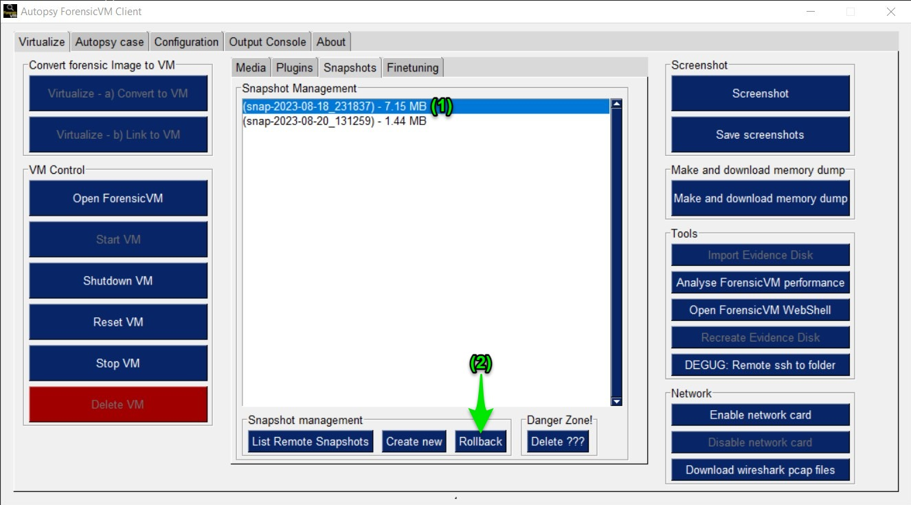
The data portal is classified based on its type of license. The open source license based data portals are known as open data portals which are used by many government organizations and academic institutions. The data portal sometimes lists a wide variety of subtypes of datasets pertaining to many machine learning applications. Figure 1: Snapshots in ForensicVM: A Crucial Asset for Investigators — ForensicVM ...
The data portals which are suitable for a specific subtype of machine learning application are listed in the subsequent sections. **RTP set** – 35,087 stationary-point geometries (reactant, transition state and product) drawn from 11,961 elementary reactions, each labeled with density-functional energies, atomic forces and full Hessian matrices at the ωB97X-D/6-31G(d) level. **IRC set** – 34,248 structures along 600 minimum-energy reaction paths, used to test extrapolation beyond trained stationary points. **NMS set** – 62,527 off-equilibrium geometries generated by normal-mode sampling to probe model robustness under thermal perturbations. The collection underpins the study Does Hessian Data Improve the Performance of Machine Learning Potentials? and was used to train and benchmark the machine-learning interatomic potentials reported therein. The dataset itself is distributed under a CC licence via Figshare.
OpenML: Web platform with Python, R, Java, and other APIs for downloading hundreds of machine learning datasets, evaluating algorithms on datasets, and benchmarking algorithm performance against dozens of other algorithms. PMLB: A large, curated repository of benchmark datasets for evaluating supervised machine learning algorithms. Provides classification and regression datasets in a standardized format that are accessible through a Python API. Metatext NLP: https://metatext.io/datasets web repository maintained by community, containing nearly 1000 benchmark datasets, and counting. Provides many tasks from classification to QA, and various languages from English, Portuguese to Arabic. Appen: Off The Shelf and Open Source Datasets hosted and maintained by the company. These biological, image, physical, question answering, signal, sound, text, and video resources number over 250 and can be applied to over 25 different use cases.
Lidar (, an acronym of light detection and ranging or laser imaging, detection, and ranging, often stylized LiDAR) is a method for determining ranges by targeting an object or a surface with a laser and measuring the time for the reflected light to return to the optical receiver. Lidar may operate in a fixed direction (e.g., vertical) or it may scan directions, in a special combination of 3D scanning and laser scanning.
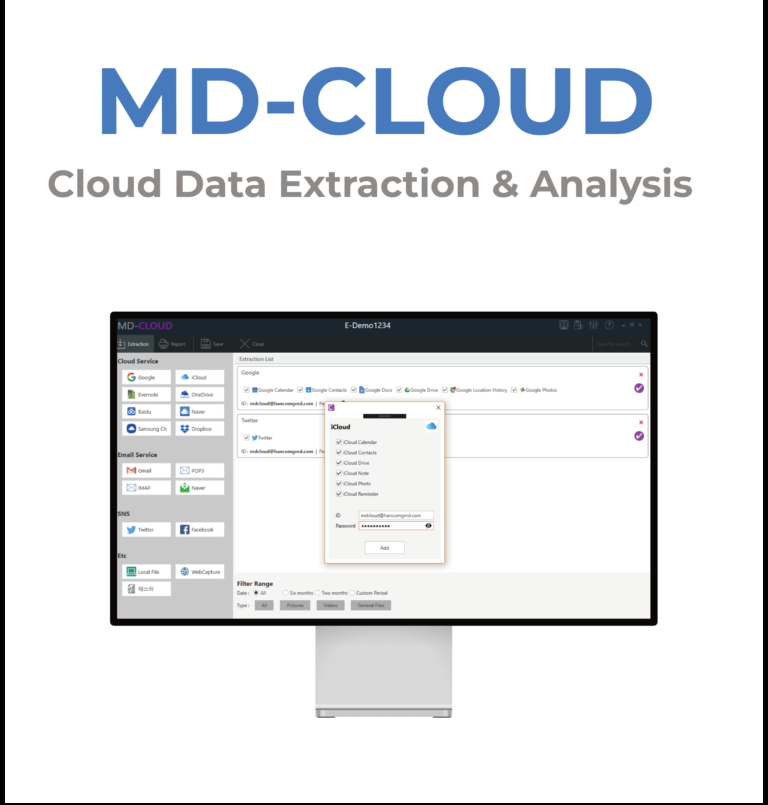
Figure 2: GMDSOFT - Dynamic Solutions-Best Forensic Software Company In Bangladesh LiDAR is used within terrestrial, airborne, and mobile equipment around the globe. It is commonly used to make high-resolution maps, with applications in surveying, geodesy, geomatics, archaeology, geography, geology, geomorphology, seismology, forestry, atmospheric physics, laser guidance, airborne laser swathe mapping (ALSM), and laser altimetry. It is used to make digital 3D representations of areas on the Earth's surface and ocean bottom of the intertidal and near coastal zone by varying the wavelength of light. It has also been increasingly used in control and navigation for autonomous cars and for the helicopter Ingenuity on its record-setting flights over the terrain of Mars. Lidar has since been used extensively for atmospheric research and meteorology. Lidar instruments fitted to aircraft and satellites carry out surveying and mapping – a recent example being the U.S. Geological Survey Experimental Advanced Airborne Research Lidar. NASA has identified lidar as a key technology for enabling autonomous precision safe landing of future robotic and crewed lunar-landing vehicles.
Lidar uses ultraviolet, visible, or near infrared light to image objects. It can target a wide range of materials, including non-metallic objects, rocks, rain, chemical compounds, aerosols, clouds and even single molecules. A narrow laser beam can map physical features with very high resolutions; for example, an aircraft can map terrain at 30-centimetre (12 in) resolution or better. Wavelengths vary to suit the target: from about 10 micrometers (infrared) to approximately 250 nanometers (ultraviolet). Typically, light is reflected via backscattering, as opposed to pure reflection one might find with a mirror. Different types of scattering are used for different lidar applications: most commonly Rayleigh scattering, Mie scattering, Raman scattering, and fluorescence. Suitable combinations of wavelengths can allow remote mapping of atmospheric contents by identifying wavelength-dependent changes in the intensity of the returned signal. The name "photonic radar" is sometimes used to mean visible-spectrum range finding like lidar, although photonic radar more strictly refers to radio-frequency range finding using photonics components. A lidar determines the distance of an object or a surface with the formula: d = c ⋅ t 2 {\displaystyle d={\frac {c\cdot t}{2}}} where c is the speed of light, d is the distance between the detector and the object or surface being detected, and t is the time spent for the laser light to travel to the object or surface being detected, then travel back to the detector. The two kinds of lidar detection schemes are "incoherent" or direct energy detection (which principally measures amplitude changes of the reflected light) and coherent detection (best for measuring Doppler shifts, or changes in the phase of the reflected light). Coherent systems generally use optical heterodyne detection. This is more sensitive than direct detection and allows them to operate at much lower power, but requires more complex transceivers. Both types employ pulse models: either micropulse or high energy. Micropulse systems utilize intermittent bursts of energy. They developed as a result of ever-increasing computer power, combined with advances in laser technology. They use considerably less energy in the laser, typically on the order of one microjoule, and are often "eye-safe", meaning they can be used without safety precautions. High-power systems are common in atmospheric research, where they are widely used for measuring atmospheric parameters: the height, layering and densities of clouds, cloud particle properties (extinction coefficient, backscatter coefficient, depolarization), temperature, pressure, wind, humidity, and trace gas concentration (ozone, methane, nitrous oxide, etc.).
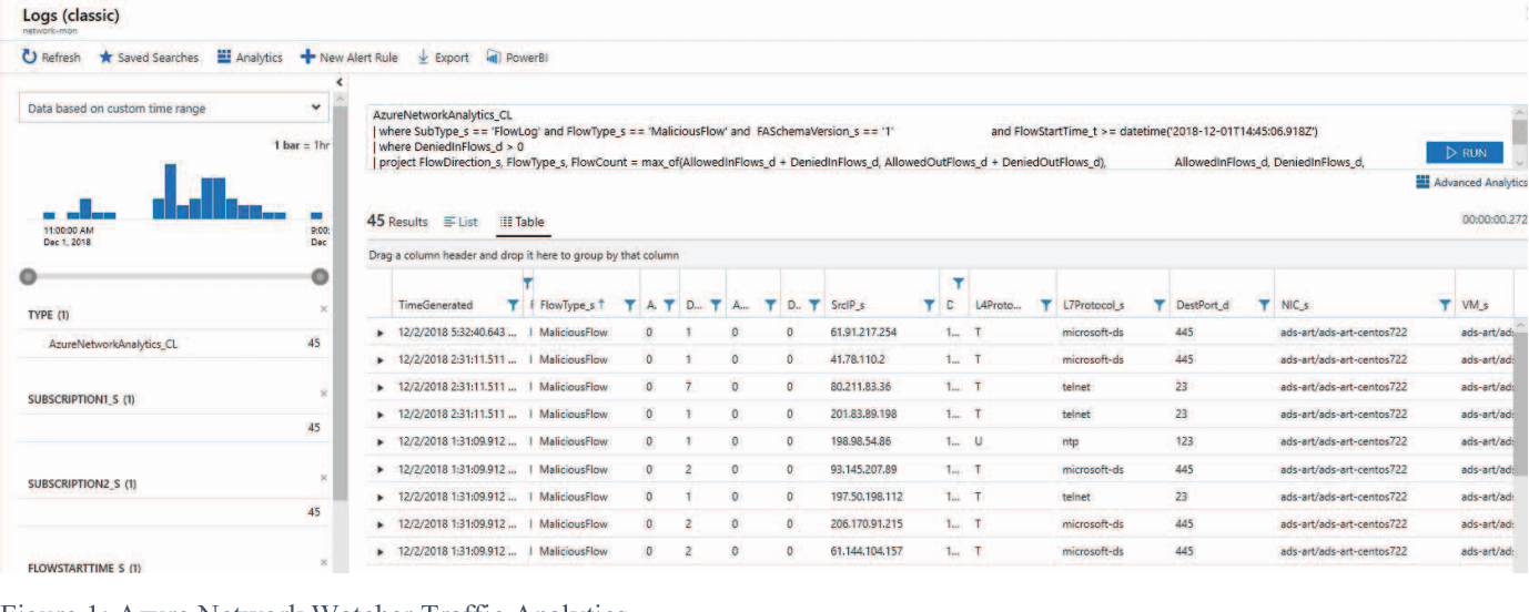
Figure 3: Figure 1 from Forensic Analysis of Cloud Virtual Environments ... Lidar applications can be divided into airborne and terrestrial types. The two types require scanners with varying specifications based on the data's purpose, the size of the area to be captured, the range of measurement desired, the cost of equipment, and more. Spaceborne platforms are also possible, using satellite laser altimetry. Airborne lidar (also airborne laser scanning) is when a laser scanner, while attached to an aircraft during flight, creates a 3D point cloud model of the landscape. This is currently the most detailed and accurate method of creating digital elevation models, replacing photogrammetry. One major advantage in comparison with photogrammetry is the ability to filter out reflections from vegetation from the point cloud model to create a digital terrain model which represents ground surfaces such as rivers, paths, cultural heritage sites, etc., which are concealed by trees. Within the category of airborne lidar, there is sometimes a distinction made between high-altitude and low-altitude applications, but the main difference is a reduction in both accuracy and point density of data acquired at higher altitudes. Airborne lidar can also be used to create bathymetric models in shallow water.
The main constituents of airborne lidar include digital elevation models (DEM) and digital surface models (DSM). The points and ground points are the vectors of discrete points while DEM and DSM are interpolated raster grids of discrete points. The process also involves capturing of digital aerial photographs. To interpret deep-seated landslides for example, under the cover of vegetation, scarps, tension cracks or tipped trees airborne lidar is used. Airborne lidar digital elevation models can see through the canopy of forest cover, perform detailed measurements of scarps, erosion and tilting of electric poles. Airborne lidar data is processed using a toolbox called Toolbox for Lidar Data Filtering and Forest Studies (TIFFS) for lidar data filtering and terrain study software. The data is interpolated to digital terrain models using the software. The laser is directed at the region to be mapped and each point's height above the ground is calculated by subtracting the original z-coordinate from the corresponding digital terrain model elevation. Based on this height above the ground the non-vegetation data is obtained which may include objects such as buildings, electric power lines, flying birds, insects, etc. The rest of the points are treated as vegetation and used for modeling and mapping. Within each of these plots, lidar metrics are calculated by calculating statistics such as mean, standard deviation, skewness, percentiles, quadratic mean, etc.
Multiple commercial lidar systems for unmanned aerial vehicles are currently on the market. These platforms can systematically scan large areas, or provide a cheaper alternative to manned aircraft for smaller scanning operations. The airborne lidar bathymetric technological system involves the measurement of time of flight of a signal from a source to its return to the sensor. The data acquisition technique involves a sea floor mapping component and a ground truth component that includes video transects and sampling. It works using a green spectrum (532 nm) laser beam. Two beams are projected onto a fast rotating mirror, which creates an array of points. One of the beams penetrates the water and also detects the bottom surface of the water under favorable conditions. Water depth measurable by lidar depends on the clarity of the water and the absorption of the wavelength used. Water is most transparent to green and blue light, so these will penetrate deepest in clean water. Blue-green light of 532 nm produced by frequency doubled solid-state IR laser output is the standard for airborne bathymetry. This light can penetrate water but pulse strength attenuates exponentially with distance traveled through the water. Lidar can measure depths from about 0.9 to 40 m (3 to 131 ft), with vertical accuracy in the order of 15 cm (6 in).
The surface reflection makes water shallower than about 0.9 m (3 ft) difficult to resolve, and absorption limits the maximum depth. Turbidity causes scattering and has a significant role in determining the maximum depth that can be resolved in most situations, and dissolved pigments can increase absorption depending on wavelength. Other reports indicate that water penetration tends to be between two and three times Secchi depth. Bathymetric lidar is most useful in the 0–10 m (0–33 ft) depth range in coastal mapping. On average in fairly clear coastal seawater lidar can penetrate to about 7 m (23 ft), and in turbid water up to about 3 m (10 ft). An average value found by Saputra et al, 2021, is for the green laser light to penetrate water about one and a half to two times Secchi depth in Indonesian waters. Water temperature and salinity have an effect on the refractive index which has a small effect on the depth calculation. The data obtained shows the full extent of the land surface exposed above the sea floor. This technique is extremely useful as it will play an important role in the major sea floor mapping program. The mapping yields onshore topography as well as underwater elevations. Sea floor reflectance imaging is another solution product from this system which can benefit mapping of underwater habitats. This technique has been used for three-dimensional image mapping of California's waters using a hydrographic lidar. Airborne lidar systems were traditionally able to acquire only a few peak returns, while more recent systems acquire and digitize the entire reflected signal.
Scientists analysed the waveform signal for extracting peak returns using Gaussian decomposition. Zhuang et al, 2017 used this approach for estimating aboveground biomass. Handling the huge amounts of full-waveform data is difficult. Therefore, Gaussian decomposition of the waveforms is effective, since it reduces the data and is supported by existing workflows that support interpretation of 3D point clouds. Recent studies investigated voxelisation. The intensities of the waveform samples are inserted into a voxelised space (3D grayscale image) building up a 3D representation of the scanned area. Related metrics and information can then be extracted from that voxelised space. Structural information can be extracted using 3D metrics from local areas and there is a case study that used the voxelisation approach for detecting dead standing eucalypt trees in Australia. Terrestrial applications of lidar (also terrestrial laser scanning) happen on the Earth's surface and can be either stationary or mobile. Stationary terrestrial scanning is most common as a survey method, for example in conventional topography, monitoring, cultural heritage documentation and forensics. The 3D point clouds acquired from these types of scanners can be matched with digital images taken of the scanned area from the scanner's location to create realistic looking 3D models in a relatively short time when compared to other technologies. Each point in the point cloud is given the colour of the pixel from the image taken at the same location and direction as the laser beam that created the point. Terrestrial lidar mapping involves a process of occupancy grid map generation. The process involves an array of cells divided into grids which employ a process to store the height values when lidar data falls into the respective grid cell. A binary map is then created by applying a particular threshold to the cell values for further processing. The next step is to process the radial distance and z-coordinates from each scan to identify which 3D points correspond to each of the specified grid cell leading to the process of data formation. Mobile lidar (also mobile laser scanning) is when two or more scanners are attached to a moving vehicle to collect data along a path. These scanners are almost always paired with other kinds of equipment, including GNSS receivers and IMUs. One example application is surveying streets, where power lines, exact bridge heights, bordering trees, etc. all need to be taken into account. Instead of collecting each of these measurements individually in the field with a tachymeter, a 3D model from a point cloud can be created where all of the measurements needed can be made, depending on the quality of the data collected. This eliminates the problem of forgetting to take a measurement, so long as the model is available, reliable and has an appropriate level of accuracy.
There are a wide variety of lidar applications, in addition to the applications listed below, as it is often mentioned in national lidar dataset programs. These applications are largely determined by the range of effective object detection; resolution, which is how accurately the lidar identifies and classifies objects; and reflectance confusion, meaning how well the lidar can see something in the presence of bright objects, like reflective signs or bright sun. Companies are working to cut the cost of lidar sensors, currently anywhere from about US$1,200 to more than $12,000. Lower prices will make lidar more attractive for new markets.
Lidar can also help to create high-resolution digital elevation models (DEMs) of archaeological sites that can reveal micro-topography that is otherwise hidden by vegetation. The intensity of the returned lidar signal can be used to detect features buried under flat vegetated surfaces such as fields, especially when mapping using the infrared spectrum. The presence of these features affects plant growth and thus the amount of infrared light reflected back. For example, at Fort Beauséjour – Fort Cumberland National Historic Site, Canada, lidar discovered archaeological features related to the siege of the Fort in 1755. Features that could not be distinguished on the ground or through aerial photography were identified by overlaying hill shades of the DEM created with artificial illumination from various angles. Another example is work at Caracol by Arlen Chase and his wife Diane Zaino Chase. In 2012, lidar was used to search for the legendary city of La Ciudad Blanca or "City of the Monkey God" in the La Mosquitia region of the Honduran jungle. During a seven-day mapping period, evidence was found of man-made structures. In June 2013, the rediscovery of the city of Mahendraparvata was announced. In southern New England, lidar was used to reveal stone walls, building foundations, abandoned roads, and other landscape features obscured in aerial photography by the region's dense forest canopy. In Cambodia, lidar data were used by Damian Evans and Roland Fletcher to reveal anthropogenic changes to Angkor landscape. In 2012, lidar revealed that the Purépecha settlement of Angamuco in Michoacán, Mexico had about as many buildings as today's Manhattan; while in 2016, its use in mapping ancient Maya causeways in northern Guatemala, revealed 17 elevated roads linking the ancient city of El Mirador to other sites. In 2018, archaeologists using lidar discovered more than 60,000 man-made structures in the Maya Biosphere Reserve, a "major breakthrough" that showed the Maya civilization was much larger than previously thought. In 2024, archaeologists using lidar discovered a new Maya site, Valeriana, as well as the Upano Valley sites in Ecuador.
Initially, based on ruby lasers, lidar for meteorological applications was constructed shortly after the invention of the laser and represents one of the first applications of laser technology. Lidar technology has since expanded vastly in capability and lidar systems are used to perform a range of measurements that include profiling clouds, measuring winds, studying aerosols, and quantifying various atmospheric components. Atmospheric components can in turn provide useful information including surface pressure (by measuring the absorption of oxygen or nitrogen), greenhouse gas emissions (carbon dioxide and methane), photosynthesis (carbon dioxide), fires (carbon monoxide), and humidity (water vapor). Atmospheric lidars can be either ground-based, airborne or satellite-based depending on the type of measurement. Atmospheric lidar remote sensing works in two ways: by measuring backscatter from the atmosphere, and by measuring the scattered reflection off the ground (when the lidar is airborne) or other hard surface. Backscatter from the atmosphere directly gives a measure of clouds and aerosols. Other derived measurements from backscatter such as winds or cirrus ice crystals require careful selecting of the wavelength and/or polarization detected. Doppler lidar and Rayleigh Doppler lidar are used to measure temperature and wind speed along the beam by measuring the frequency of the backscattered light. The Doppler broadening of gases in motion allows the determination of properties via the resulting frequency shift. Scanning lidars, such as NASA's conical-scanning HARLIE, have been used to measure atmospheric wind velocity. The ESA wind mission ADM-Aeolus will be equipped with a Doppler lidar system in order to provide global measurements of vertical wind profiles. A doppler lidar system was used in the 2008 Summer Olympics to measure wind fields during the yacht competition. Doppler lidar systems are also now beginning to be successfully applied in the renewable energy sector to acquire wind speed, turbulence, wind veer, and wind shear data. Both pulsed and continuous wave systems are being used. Pulsed systems use signal timing to obtain vertical distance resolution, whereas continuous wave systems rely on detector focusing. The term eolics has been proposed to describe the collaborative and interdisciplinary study of wind using computational fluid mechanics simulations and Doppler lidar measurements. The ground reflection of an airborne lidar gives a measure of surface reflectivity (assuming the atmospheric transmittance is well known) at the lidar wavelength, however, the ground reflection is typically used for making absorption measurements of the atmosphere. "Differential absorption lidar" (DIAL) measurements utilize two or more closely spaced (less than 1 nm) wavelengths to factor out surface reflectivity as well as other transmission losses, since these factors are relatively insensitive to wavelength. When tuned to the appropriate absorption lines of a particular gas, DIAL measurements can be used to determine the concentration (mixing ratio) of that particular gas in the atmosphere. This is referred to as an integrated path differential absorption (IPDA) approach, since it is a measure of the integrated absorption along the entire lidar path. IPDA lidars can be either pulsed or CW and typically use two or more wavelengths. IPDA lidars have been used for remote sensing of carbon dioxide and methane. Synthetic array lidar allows imaging lidar without the need for an array detector. It can be used for imaging Doppler velocimetry, ultra-fast frame rate imaging (millions of frames per second), as well as for speckle reduction in coherent lidar. An extensive lidar bibliography for atmospheric and hydrospheric applications is given by Grant.
THOR is a laser designed toward measuring Earth's atmospheric conditions. The laser enters a cloud cover and measures the thickness of the return halo. The sensor has a fiber optic aperture with a width of 7+1⁄2 inches (19 cm) that is used to measure the return light. 2. System Architecture & Core Working Principles Lidar has also found many applications for mapping natural and managed landscapes such as forests, wetlands, and grasslands. Canopy heights, biomass measurements, and leaf area can all be studied using airborne lidar systems. Similarly, lidar is also used by many industries, including Energy and Railroad, and the Department of Transportation as a faster way of surveying. Topographic maps can also be generated readily from lidar, including for recreational use such as in the production of orienteering maps. Lidar has also been applied to estimate and assess the biodiversity of plants, fungi, and animals. Using southern bull kelp in New Zealand, coastal lidar mapping data has been compared with population genomic evidence to form hypotheses regarding the occurrence and timing of prehistoric earthquake uplift events.
In Japan, differential absorption lidar (DIAL) and Raman lidar technologies are being developed to improve the accuracy of flood forecasting and rainfall prediction. A research by several companies, universities, and institutes, led by Kyushu University is conducting work on meteorological sensing and flood-risk modelling under a government program. Observing the vertical distribution of water vapor, temperature, wind direction, and wind speed using lidar; Integrating this data with satellite observations and upper-air weather maps to create new meteorological data sets; Applying artificial intelligence models to simulate and predict precipitation, river flows, and flood risk. In May 2025, EKO Instruments began a field study on Goto Fukue Island, Nagasaki Prefecture, using a Micropulse DIAL lidar system provided by the National Center for Atmospheric Research (NSF NCAR). The study compares DIAL performance with existing Raman lidar systems. In addition, EKO Instruments. Co. Ltd. signed a technology license agreement in February 2025 with Montana State University, NSF NCAR, and NASA, covering key DIAL-related patents.
Discontinuity orientation Discontinuity spacing and RQD Discontinuity aperture Discontinuity persistence Discontinuity roughness Water infiltration Some of these properties have been used to assess the geomechanical quality of the rock mass through the RMR index. Moreover, as the orientations of discontinuities can be extracted using the existing methodologies, it is possible to assess the geomechanical quality of a rock slope through the SMR index. In addition to this, the comparison of different 3D point clouds from a slope acquired at different times allows researchers to study the changes produced on the scene during this time interval as a result of rockfalls or any other landsliding processes.
Airborne lidar sensors are used by companies in the remote sensing field. They can be used to create a DTM (digital terrain model) or DEM (digital elevation model); this is quite a common practice for larger areas as a plane can acquire 3–4 km (2–2+1⁄2 mi) wide swaths in a single flyover. Greater vertical accuracy of below 50 mm (2 in) can be achieved with a lower flyover, even in forests, where it is able to give the height of the canopy as well as the ground elevation. Typically, a GNSS receiver configured over a georeferenced control point is needed to link the data in with the WGS (World Geodetic System).
Lidar is also in use in hydrographic surveying. Depending upon the clarity of the water lidar can measure depths from 0.9 to 40 m (3 to 131 ft) with a vertical accuracy of 15 cm (6 in) and horizontal accuracy of 2.5 m (8 ft). Agricultural robots have been used for a variety of purposes ranging from seed and fertilizer dispersions, sensing techniques as well as crop scouting for the task of weed control. Lidar can help determine where to apply costly fertilizer. It can create a topographical map of the fields and reveal slopes and sun exposure of the farmland. Researchers at the Agricultural Research Service used this topographical data with the farmland yield results from previous years, to categorize land into zones of high, medium, or low yield. This indicates where to apply fertilizer to maximize yield. Lidar is now used to monitor insects in the field.
The use of lidar can detect the movement and behavior of individual flying insects, with identification down to sex and species. In 2017 a patent application was published on this technology in the United States, Europe, and China. Another application is crop mapping in orchards and vineyards, to detect foliage growth and the need for pruning or other maintenance, detect variations in fruit production, or count plants. Lidar is useful in GNSS-denied situations, such as nut and fruit orchards, where foliage causes interference for agriculture equipment that would otherwise utilize a precise GNSS fix. Lidar sensors can detect and track the relative position of rows, plants, and other markers so that farming equipment can continue operating until a GNSS fix is reestablished. Controlling weeds requires identifying plant species. This can be done by using 3D lidar and machine learning. Lidar produces plant contours as a "point cloud" with range and reflectance values. This data is transformed, and features are extracted from it. If the species is known, the features are added as new data. The species is labelled and its features are initially stored as an example to identify the species in the real environment. This method is efficient because it uses a low-resolution lidar and supervised learning. It includes an easy-to-compute feature set with common statistical features which are independent of the plant size.
Lidar systems have also been applied to improve forestry management. Measurements are used to take inventory in forest plots as well as calculate individual tree heights, crown width and crown diameter. Other statistical analysis use lidar data to estimate total plot information such as canopy volume, mean, minimum and maximum heights, vegetation cover, biomass, and carbon density. Aerial lidar was used to map the bush fires in Australia in early 2020. The data was manipulated to view bare earth, and identify healthy and burned vegetation.
Lidar has been used in the railroad industry to generate asset health reports for asset management and by departments of transportation to assess their road conditions. CivilMaps.com is a leading company in the field. Lidar has been used in adaptive cruise control (ACC) systems for automobiles. Systems such as those by Siemens, Hella, Ouster and Cepton use a lidar device mounted on the front of the vehicle, such as the bumper, to monitor the distance between the vehicle and any vehicle in front of it. In the event where the vehicle in front slows down or is too close, the ACC applies the brakes to slow the vehicle. When the road ahead is clear, the ACC allows the vehicle to accelerate to a speed preset by the driver. Refer to the Military section above for further examples. A lidar-based device, the Ceilometer, is used at airports worldwide to measure the height of clouds on runway approach paths.
In April 2025, Dallas Fort Worth International Airport announced the deployment of a lidar-based platform for real-time monitoring of passenger and vehicle flows. Autonomous vehicles may use lidar for obstacle detection and avoidance to navigate safely through environments. The introduction of lidar was a pivotal occurrence that was the key enabler behind Stanley, the first autonomous vehicle to successfully complete the DARPA Grand Challenge. Point cloud output from the lidar sensor provides the necessary data for robot software to determine where potential obstacles exist in the environment and where the robot is in relation to those potential obstacles. Singapore's Singapore-MIT Alliance for Research and Technology (SMART) is actively developing technologies for autonomous lidar vehicles. The very first generations of automotive adaptive cruise control systems used only lidar sensors. In transportation systems, to ensure vehicle and passenger safety and to develop electronic systems that deliver driver assistance, understanding the vehicle and its surrounding environment is essential. Lidar systems play an important role in the safety of transportation systems. Many electronic systems which enhance driver assistance and vehicle safety such as adaptive cruise control (ACC), emergency brake assist, and anti-lock braking system (ABS) depend on the detection of a vehicle's environment to act autonomously or semi-autonomously. Lidar mapping and estimation achieve this.
Current lidar systems use rotating hexagonal mirrors which split the laser beam. The upper three beams are used for vehicle and obstacles ahead, and the lower beams are used to detect lane markings and road features. The major advantage of using lidar is that the spatial structure is obtained and this data can be fused with other sensors such as radar, etc. to get a better picture of the vehicle environment in terms of static and dynamic properties of the objects present in the environment.
Conversely, a significant issue with lidar is the difficulty in reconstructing point cloud data in poor weather conditions. In heavy rain, for example, the light pulses emitted from the lidar system are partially reflected off of rain droplets which adds noise to the data, called 'echoes'. Obstacle detection and road environment recognition using lidar, proposed by Kun Zhou et al. not only focuses on object detection and tracking but also recognizes lane marking and road features. As mentioned earlier, the lidar systems use rotating hexagonal mirrors that split the laser beam into six beams. The upper three layers are used to detect the forward objects such as vehicles and roadside objects. The sensor is made of weather-resistant material. The data detected by lidar are clustered to several segments and tracked by Kalman filter. Data clustering here is done based on characteristics of each segment based on object model, which distinguish different objects such as vehicles, signboards, etc.
These characteristics include the dimensions of the object, etc. The reflectors on the rear edges of vehicles are used to differentiate vehicles from other objects. Object tracking is done using a two-stage Kalman filter considering the stability of tracking and the accelerated motion of objects Lidar reflective intensity data is also used for curb detection by making use of robust regression to deal with occlusions. Road marking is detected using a modified Otsu method by distinguishing rough and shiny surfaces. Roadside reflectors that indicate lane border are sometimes hidden due to various reasons. Therefore, other information is needed to recognize the road border. The lidar used in this method can measure the reflectivity from the object. Hence, with this data the road border can also be recognized. Also, the usage of a sensor with a weather-robust head helps to detect the objects even in bad weather conditions. Canopy height model before and after a flood is a good example.
Lidar can detect highly detailed canopy height data as well as its road border. Lidar measurements help identify the spatial structure of the obstacle. This helps distinguish objects based on size and estimate the impact of driving over it. Lidar systems provide better range and a large field of view, which helps in detecting obstacles on the curves. This is one of its major advantages over radar systems, which have a narrower field of view. The fusion of lidar measurement with different sensors makes the system robust and useful in real-time applications, since lidar-dependent systems cannot estimate the dynamic information about the detected object. It has been shown that lidar can be manipulated, such that self-driving cars are tricked into taking evasive action.
Computer stereo vision has shown promise as an alternative to lidar for close-range applications. It is significantly more cost effective when appropriate. Outsight (25 May 2023). "Understanding the Basics of 3D LiDAR Technology". Outsight Insights. National Oceanic and Atmospheric Administration (NOAA) (15 April 2020). "What is LIDAR?". NOAA's National Ocean Service. The USGS Center for LIDAR Information Coordination and Knowledge (CLICK) – A website intended to "facilitate data access, user coordination and education of lidar remote sensing for scientific needs." How snapshot chains store evidence across multiple files, how to correctly flatten or traverse them, and how to extract both disk and memory artifacts from every major hypervisor platform.
Virtual machines have become primary evidence sources in corporate investigations, malware analysis, cloud incident response, and criminal cases where suspects used VMs to compartmentalize activity or attempt to hide evidence. A virtual machine is not just a disk image — it is an entire computer system captured in files. Those files include the disk, the memory state at each snapshot point, the hardware configuration, and a complete history of changes recorded in delta layers stretching back through potentially years of snapshots. As the VMware Security blog observes, the ability to save machine state to disk creates a natural synergy between virtualization and memory forensics — and in some cases, it is possible to collect a memory dump of a running virtualized machine without interrupting its execution. Understanding how to acquire, flatten, and analyze every layer of a VM’s file structure is what determines how much of that history is recoverable.
This guide covers the file structure of virtual machines across VMware, Hyper-V, VirtualBox, and KVM/QEMU; how snapshot chains work and how to traverse them without destroying historical evidence; the correct acquisition procedures for both running and suspended VMs; how to flatten snapshot chains into analyzable images; how to extract and analyze VM memory files; the critical tool differences between vmss2core, Volatility, and VBoxManage for memory conversion; and how to locate and recover deleted VM artifacts on the host system.
Understanding what each VMware file contains is the prerequisite for knowing which files to acquire and in what order. A typical VMware virtual machine directory contains the following files: Do not acquire only the VMDK. The .vmx configuration, .vmsd snapshot database, .log files, .nvram, and any .vmsn/.vmss files are all independently forensically significant. Acquire the entire VM directory as a unit. Use the host disk image as the source wherever possible, as copying individual VM files alters their MACE timestamps on the host filesystem.
When a snapshot is taken in VMware, the base disk ( -flat.vmdk ) is frozen and becomes read-only. VMware creates a new delta VMDK file (typically named with a sequential number like -000001.vmdk and -000001-delta.vmdk ) that will record only the sectors that change after the snapshot. The guest OS continues writing to the delta. The base disk remains unchanged. When a second snapshot is taken, the first delta is also frozen and a second delta is created ( -000002.vmdk / -000002-delta.vmdk ) that records changes after the second snapshot. The chain continues: base → delta1 → delta2 → … → current delta. Each level represents the disk state at the moment that snapshot was taken plus all changes up to the next snapshot.
Each snapshot delta represents the disk state at a specific point in time. If the suspect deleted files between snapshots, those deleted files may still exist in an earlier delta layer — deleted at the active layer but intact in the snapshot that predates the deletion. If malware was installed after a snapshot was taken, the base disk is clean and only the delta contains the malware. The snapshot history is a timeline of the VM’s disk state, and every layer is independently analyzable.
3. Software Implementation, Frameworks & Protocols The .vmsd file is the index of this history. It records each snapshot’s name, UID, creation time, and parent-child relationships. Read it to understand the complete snapshot tree before beginning acquisition. For a running VMware VM, the recommended forensic acquisition approach is to suspend the VM rather than imaging it while running. As Paul Henry, a senior SANS Institute instructor, explains in the SANS Digital Forensics blog, imaging a running VM is impractical from a forensics perspective because the VMDK will be undergoing constant change, making it impossible to validate image integrity through before-and-after hash comparison. Suspension freezes the VM state, creates a .vmss file containing the guest’s complete memory, and pauses all disk writes. The result is a static, consistent snapshot of both disk and memory that can be imaged with verifiable hash values.
The SANS blog further notes that the -flat.vmdk file is an abstraction of a physical disk contained within a file, and that suspending the VM provides an additional forensic bonus: the .vmss file represents a snapshot of the VM’s RAM at the moment of suspension. This file can contain valuable forensic evidence of what was occurring in the running VM’s memory and should be imaged alongside the VMDK.
After suspension, the VM directory contains the current disk state (base + all deltas) and the .vmss suspended state file with memory. These files can now be acquired. For production VMs that cannot be suspended, take a snapshot with memory capture enabled. This creates a .vmem file (raw memory dump) and a delta VMDK that captures the disk state at the snapshot moment. The running VM continues on a new delta layer while the snapshotted state is preserved for acquisition.
In vSphere client: right-click VM > Snapshot > Take Snapshot > check Snapshot the virtual machine’s memory . Via command line: Once the snapshot is created, the parent disk (the state at snapshot time) is frozen and the .vmem file contains the memory state at that moment. The running VM continues on the new delta. Acquire the snapshot files immediately — the delta will grow as the VM continues to run, but the snapshotted state is frozen.
For forensic analysis, it is often necessary to produce a single flat disk image representing the VM’s state at a specific point in the snapshot chain rather than analyzing the individual layers separately. Flattening merges the base disk and all or some delta layers into a single contiguous image. Never flatten or modify the original VM files. Copy the entire VM directory to the forensic workstation before any flattening operation. The originals must remain unmodified so that each individual snapshot layer can be examined independently.
vmware-vdiskmanager is included with VMware Workstation and VMware Fusion. On ESXi, the equivalent is vmkfstools . X-Ways Forensics can import VMDK snapshot chains incrementally without flattening, which preserves the ability to see exactly which sectors changed between each snapshot. As documented in DFIR practitioner workflows, X-Ways requires that VMDK files be opened in chronological order — base disk first, then each delta in sequence. If you attempt to import a delta file before its parent, X-Ways returns an error stating that the corresponding parent must be opened first in order of last-modified dates, oldest first, skipping none. Once loaded in order, X-Ways presents each snapshot layer for independent analysis, allowing the examiner to compare filesystem states between snapshots and identify exactly when files were created, modified, or deleted.
When EnCase or FTK Imager is pointed directly at a delta VMDK file, the tool converts only that delta layer — not the complete chain from the base disk through all deltas. This was demonstrated and documented in the 2012 RIT research paper by Hirwani et al., which found that when EnCase is pointed to a later snapshot, it only converts the delta that is created after the snapshot, not the full chain. The result is a partial image containing only the changed blocks from that delta, not a complete disk image. To analyze the full disk state using EnCase or FTK Imager, flatten the chain first using vmware-vdiskmanager or vmkfstools , then point the forensic tool at the resulting flat VMDK. The same RIT study confirmed that both EnCase and FTK Imager can safely convert base (non-snapshot) VMDK files to raw DD format with matching hash values.
After flattening, the -flat.vmdk file is a raw disk image in the same format as a DD image from a physical drive. It can be imaged directly with FTK Imager, dc3dd, or any tool that accepts raw files as input. If the flat VMDK still has the descriptor file wrapper and needs to be converted to a plain raw image for tools that expect only raw binary: The .vmem file is a raw dump of the guest VM’s physical memory at the time the snapshot was taken. It is one of the most valuable forensic artifacts in a VM investigation because it contains the complete in-memory state of the guest OS: running processes, network connections, loaded kernel modules, decrypted credentials, and any in-memory malware.
The .vmss file is the suspended state file created when a VM is suspended. Unlike a memory-only .vmem dump, the .vmss file also contains the VM hardware state (CPU registers, device state) alongside the memory contents. Volatility supports .vmss files directly as well: Each snapshot’s state file ( .vmsn ) describes the VM configuration at that snapshot moment. If the snapshot was taken with memory enabled, the .vmsn file references the memory data. The VMSD file records which .vmsn corresponds to which snapshot in the chain. Read the .vmsd to map snapshot names and creation times to their corresponding .vmsn and delta VMDK files: An important implementation detail that frequently causes analysis failures: on ESXi and some VMware Workstation versions, the .vmss file contains only metadata describing the memory layout, while the actual raw memory contents are stored in a separate .vmem file. Volatility 3 will issue a warning if the metadata file is missing: “No metadata file found alongside VMEM file. A VMSS or VMSN file may be required to correctly process a VMEM file.” Both files must be placed in the same directory with matching base filenames (for example, VM-Snapshot1.vmem and VM-Snapshot1.vmss ) for Volatility to correctly reconstruct the physical memory layout.
VMware provides a utility called vmss2core that converts .vmss and .vmsn checkpoint state files (with or without a companion .vmem ) into formats compatible with third-party debuggers. As described in Broadcom’s knowledge base (article 2003941), vmss2core can produce Windows crash dump files for WinDbg and Red Hat crash-compatible core files for Linux analysis. The correct flag depends on the guest OS, not the host OS: Volatility 3 can read .vmem and .vmss files directly in most cases. Use vmss2core when Volatility cannot parse the memory format (common with very large VMs exceeding 4 GB RAM on certain ESXi versions), when you need a Windows crash dump ( .dmp ) for WinDbg analysis, or when the .vmss / .vmsn file is monolithic (memory embedded within the state file rather than in a separate .vmem ). The Volatility Foundation wiki documents that some VMware products create monolithic .vmss files while others produce separate .vmem files, and the analysis workflow differs accordingly.
4. Practical Deployment, Analysis & Case Studies Hyper-V virtual machine files are organized differently from VMware but follow the same conceptual model of a base disk plus differencing layers for checkpoints. Hyper-V has two checkpoint types, as documented in Microsoft Learn. Standard Checkpoints take a snapshot of the virtual machine and virtual machine memory state at the time the checkpoint is initiated. Standard checkpoints are forensically richer because they include memory in .bin and .vsv files (or .vmrs files on Server 2016+). Production Checkpoints use VSS (Volume Shadow Copy Service) on Windows guests or filesystem freeze on Linux guests to create an application-consistent point-in-time backup of the disk without capturing memory state. According to Microsoft, production checkpoints are selected by default on Windows 10 and later. Hyper-V only offered standard checkpoints (then called snapshots) prior to Windows 10.
If memory evidence is needed from a Hyper-V checkpoint, you must explicitly configure the VM to use Standard Checkpoints before taking the checkpoint: Starting with Windows Server 2016, Hyper-V replaced the XML-based VM configuration file with a new binary format: .vmcx for configuration data and .vmrs for runtime state data. These binary files replaced the earlier .xml , .bin , and .vsv files. On Server 2016+ hosts, checkpoint state is stored in .vmcx and .vmrs files rather than .bin / .vsv . When examining a Hyper-V host, determine the Windows Server version first to know which file formats to expect.
To acquire a Hyper-V VM’s complete evidence set, acquire all related files: the base .vhdx , all .avhdx differencing disks, the .vmcx configuration, any .bin and .vsv memory files, and the VM’s log directory. The Get-VHD cmdlet traverses the parent chain of an .avhdx file to reveal the full checkpoint lineage: Hyper-V disk files can be mounted read-only on a Windows forensic workstation using PowerShell. Mounting the current .avhdx automatically resolves and traverses the parent chain, presenting the complete current disk state as a read-only volume.
Once mounted read-only, the disk appears as a drive letter in Windows. FTK Imager can then create a forensic image of the mounted disk: File > Create Disk Image > Physical Drive > select the mounted Hyper-V disk. This produces a verifiable forensic image of the complete checkpoint-resolved disk state. VirtualBox uses .vdi (Virtual Disk Image) as its native disk format. It also supports VMDK and VHD for compatibility.
Snapshots are stored as immutable parent disks with differencing .vdi files for each snapshot layer. The VM configuration is stored in an XML file ( .vbox ), which is a plain XML document readable with any text editor. It records all hardware settings, snapshot history, and disk chain references. The .vbox-prev file is a backup of the previous configuration state.
VirtualBox .sav files contain the VM’s saved state (memory and CPU state) when the VM is paused or saved. However, unlike VMware’s .vmem files, the .sav format is not a raw memory dump and cannot be analyzed directly by Volatility. VirtualBox embeds the memory data within a proprietary container alongside device state, CPU registers, and other metadata. As the Volatility Foundation wiki notes, VirtualBox does not automatically save a full RAM dump to disk when you suspend or pause a virtual machine the way other virtualization products do.
There are two supported methods for obtaining an analyzable memory image from a VirtualBox VM, both documented by Philippe Teuwen, who contributed the VirtualBox address space to Volatility: A common misconception is that VirtualBox .sav files can be fed directly to Volatility. They cannot. The .sav format wraps memory data in a proprietary structure that Volatility does not parse. You must acquire memory using VBoxManage debugvm dumpvmcore to produce an ELF64 core dump, which Volatility supports through the VirtualBoxCoreDumpElf64 address space contributed by Philippe Teuwen and included in Volatility since version 2.3.
Once a flat disk image is produced from any hypervisor, analysis proceeds using the same tools as for physical disk images. The virtual disk is treated exactly like a physical disk image: it contains a partition table, filesystems, and all the expected forensic artifacts. Volatility 3 has native support for VMware .vmem files, VMware .vmss suspended state files, and VirtualBox ELF64 core dumps (created via VBoxManage debugvm dumpvmcore ). Hyper-V .bin files require conversion to a crash dump or raw format before analysis.
KVM (Kernel-based Virtual Machine) with QEMU is the dominant hypervisor in Linux server environments and the backbone of OpenStack cloud deployments. KVM/QEMU VMs use a different file structure than the commercial hypervisors covered above, and forensic practitioners encountering Linux-hosted infrastructure need to know how to acquire and analyze these files.
KVM/QEMU typically uses qcow2 (QEMU Copy-On-Write version 2) as the native disk format. Like VMware’s VMDK and Hyper-V’s VHDX, qcow2 supports snapshots as internal layers within the same file (rather than separate delta files). Snapshots are stored as internal snapshot tables within the qcow2 image. Raw images ( .img or .raw ) are also common, particularly in production environments prioritizing I/O performance.
The virsh dump --memory-only command produces an ELF core dump that Volatility can analyze through its QemuCoreDumpElf address space. For paused or saved VMs, the save state file produced by virsh save contains compressed memory that virsh save-image-edit can help inspect, but direct analysis requires converting to a raw dump. LiME (Linux Memory Extractor) can also be loaded into the guest kernel to produce a raw memory image from within the VM, compatible with Volatility’s LimeAddressSpace .
When a VM has been deleted from the host, its files may be recoverable through forensic analysis of the host disk. This requires imaging the host disk first, then searching for VM file artifacts within the host image. VMware disk descriptor files and VMDK flat data files, VHDX files, and VDI files have recognizable file signatures. Standard file carving tools can identify these signatures in unallocated space: On a Windows host where VMware Workstation or Hyper-V Manager was used, the host registry records recently accessed VM files. These references persist even after the VM files are deleted: 5. Performance Evaluation & Extended Technical Observations Virtual machines are used for anti-forensic purposes by attackers who are aware that VM snapshots, logs, and configuration files can be examined. Investigators should be aware of the following techniques: Snapshot deletion: Deleting all snapshots removes the delta history. However, the deleted deltas may still exist in unallocated space on the host filesystem and can potentially be recovered through carving. The VMSD file, even after snapshot deletion, may retain references to deleted snapshots if the host filesystem has not been wiped.
Log manipulation: The vmware.log file records VM activity with timestamps. A forensically aware suspect may attempt to delete or truncate this file. The file may be recoverable from unallocated space, and its absence is itself an indicator of deliberate cleanup. Encrypted VM disk: VMware supports full disk encryption within the VM (BitLocker, VeraCrypt) and at the VMDK level (VMware VM Encryption, managed through vCenter key management). An encrypted VMDK appears as random data without the key. Memory forensics is the primary path to recovering keys from an encrypted VM disk — if the VM was running and encrypted volumes were mounted, the encryption keys may reside in the .vmem file. Volatility’s bitlocker plugin (community-contributed) can extract BitLocker Full Volume Encryption Keys (FVEKs) from memory images, and the truecryptmaster plugin recovers TrueCrypt/VeraCrypt master keys. For VMware VM Encryption at the hypervisor level, the key is managed by a Key Management Server (KMS) and is not stored within the VM files themselves — the KMS administrator must provide the key or the encryption must be removed at the vCenter level before acquisition.
VM disk wiping and secure erase: A suspect may wipe the VM’s virtual disk from within the guest OS. However, because virtual disks are thin-provisioned files on the host filesystem, the wiped sectors may not be zeroed on the host’s physical storage. Carving the host disk’s unallocated space may recover fragments of the original VM disk content that the thin-provisioning layer has not yet reclaimed.
Nested virtualization and VM in VM: A VM may contain another VM. The outer VM’s disk image contains the files of the inner VM, which must then be recursively analyzed. This nesting can go multiple levels deep, though performance constraints typically limit it to two levels in practice. VM acquisition documentation must record the complete file inventory and the steps taken to produce the forensic image, because a third party must be able to reproduce the acquisition from the documented steps alone.
VM file inventory: A complete list of every file in the VM directory with filename, size, and hash value for each file individually (not just the final imaged disk). This records the state of the entire VM directory at the time of acquisition. The .vmsd snapshot database, .vmx configuration, .log files, and all .vmem/.vmss/.vmsn files must all be individually hashed and inventoried. Snapshot chain documentation: The contents of the .vmsd file must be recorded verbatim — this documents the snapshot history, names, creation times, and parent-child relationships. If the snapshot chain was flattened to produce the analysis image, the tool name, version, and exact command used must be recorded, along with the hash of the input (the delta VMDK used as the source) and the hash of the output (the flattened image).
Memory file acquisition: If .vmem or .vmss files were acquired, record the snapshot name and timestamp they correspond to (from the .vmsd), the hash of the memory file, and any tool used to convert it before Volatility analysis. Analysis image provenance: The final analysis disk image must be documented with: the source (which file or files were used to produce it), the tool and version, the hash of the output before analysis begins, and any intermediate steps (flattening, conversion) with their own tool/version/hash records.
Common questions about VM disk files, snapshot chains, memory analysis, and evidence recovery from virtual environments. The base VMDK contains the original disk state at VM creation or last consolidation. When a snapshot is taken, VMware freezes the base disk read-only and creates a new delta VMDK recording only subsequent changes. Each snapshot adds another delta layer. The current VM state is the result of applying all deltas on top of the base in order. Each snapshot represents a distinct point-in-time disk state, and the delta files are the evidence of what changed between snapshots.
Use VMware’s vmware-vdiskmanager -r [current-delta.vmdk] -t 0 [output-flat.vmdk] . This reads the entire chain from base through all deltas and writes a consolidated flat image. On ESXi, use vmkfstools -d thin -i [base.vmdk] [output.vmdk] . Always work from copies of the original files — never flatten the originals. EnCase and FTK Imager pointed directly at a delta VMDK only convert that delta, not the full chain.
The .vmem file is a raw dump of the VM guest’s physical memory at snapshot or suspension time: running processes, network connections, encryption keys, credentials, and in-memory malware. Volatility 3 reads .vmem files directly without conversion: python3 vol.py -f guest.vmem windows.info.Info . The .vmss suspended state file similarly contains memory and can be read by Volatility. Both are among the most valuable artifacts in a VM investigation.
When a Hyper-V checkpoint is taken, the base .vhdx is frozen read-only and a new .avhdx differencing disk is created. All subsequent writes go to the .avhdx. Standard checkpoints also produce .bin (memory) and .vsv (device state) files. Multiple checkpoints create a chain of .avhdx files. Mount the current .avhdx with Mount-VHD -Path [file.avhdx] -ReadOnly — PowerShell automatically resolves the full parent chain to present the complete current state.
The preferred approach is to suspend the VM (which creates a .vmss memory file and freezes all disk writes), then acquire the suspended VM files. This produces a consistent, hashable image with both disk and memory evidence. If suspension is not possible, take a snapshot with memory capture enabled. The snapshot freezes the base disk while the running VM continues on a new delta. If neither is possible, live imaging produces a valid but non-hash-verifiable acquisition that must be documented as a live acquisition.
VM files deleted from the host filesystem may be recoverable through unallocated space carving on the host disk image. VMDK, VHD/VHDX, and VDI files have recognizable signatures that carving tools can find. The plaintext .vmx configuration file and vmware.log can be found through keyword searching. Host registry artifacts (VMware recent file lists, Hyper-V event logs) record VM activity even after deletion. Image the host disk first, then carve for VM file signatures and examine host application artifacts.
No. A common misconception is that VirtualBox .sav files can be analyzed directly with Volatility, but they cannot. VirtualBox wraps memory data in a proprietary container that Volatility does not parse. To analyze VirtualBox VM memory, use VBoxManage debugvm "VMName" dumpvmcore --filename output.elf to produce an ELF64 core dump while the VM is running. Volatility supports these ELF64 core dumps through the VirtualBoxCoreDumpElf64 address space, contributed by Philippe Teuwen and included since Volatility 2.3.
This is a potential security issue, you are being redirected to https://csrc.nist.gov . Harvested Online Documentation & Reference Sources • https://en.wikipedia.org/wiki/Memory%20forensics • https://en.wikipedia.org/wiki/List%20of%20datasets%20for%20machine-learning%20research • https://en.wikipedia.org/wiki/Lidar • https://kandibrian.com/articles/virtual-machine-forensics-snapshot-extraction.html • https://csrc.nist.gov/pubs/sp/800/201/final
Extracted Research Figures & Simulation Topologies
Total 3 diagrams and telemetry visual outputs extracted directly from the complete technical documentation.
Breach Emulation & Defense Validation Architecture
Standardized testing pipeline mapping threat vectors directly into simulated inspection engines.
(AttackIQ / SafeBreach)
(Burp Suite Pro)
(Cisco Packet Tracer)
(Metasploit Engine)
(KnowBe4 Training)
Sample Simulation Code & Telemetry Log
Automated tool orchestration script and command window outputs for Cloud Virtual Machine Snapshot Forensic Analysis Tool.
[*] Metasploit Scan Running on Target Subnet for Cloud Virtual Machine Snapshot Forensic Analysis Tool... [✓] SafeBreach / AttackIQ Continuous Exposure Agent Triggered ──────────────────────────────────────────────────────────────────────── [11:48:02.104] PICUS Threat Scenario Dispatched: Lateral Movement SMB Probe [11:48:02.185] BLOCKED Endpoint EDR Detected Technique | Packet Tracer ACL Denied [11:48:02.240] CYMULATE Prevention Rate = 96.8% | SIEM Latency = 38 ms [11:48:02.312] ATTACKIQ Posture Validation: MITRE ATT&CK matrix fully validated ──────────────────────────────────────────────────────────────────────── [✓] BAS Simulation Run Complete: Defense-in-Depth Verified Across All Controls
| Simulation Platform | Simulated Threat / Scenario | Target Subsystem | Detection Latency | Security Control Status |
|---|---|---|---|---|
| Metasploit Framework | Port Reconnaissance & Fingerprinting | DMZ Gateway | 18 ms | MONITORED & DROPPED |
| AttackIQ Enterprise | Credential Access (LSASS Dump) | Windows Client | 42 ms | BLOCKED BY EDR |
| SafeBreach | Ransomware Lateral Movement | File Server Subnet | 65 ms | ISOLATED IN SANDBOX |
| Cymulate | Email Gateway Malicious Attachment | Corporate Mailbox | 120 ms | QUARANTINED |
| Picus Security | Command & Control (C2) Beaconing | Edge Firewall | 24 ms | BLOCKED BY ACL |