Complete Technical Paper Content — Credit Card Fraud Detection Using Machine Learning Python Source Code
Overview & System Context
Credit Card Fraud Detection Using Machine Learning Python Source Code: Comprehensive Web-Sourced Technical Investigation Exhaustive Research Dossier · Pure Web-Scraped Content: ~9515 Words · Real Software Screenshots: 3 1. Executive Overview & Technical Background The goal of this project is to develop a machine learning model that can accurately detect fraudulent credit card transactions using historical data. By analyzing transaction patterns, the model should be able to distinguish between normal and fraudulent activity, helping financial institutions flag suspicious behavior early and reduce potential risks.
We begin by importing the necessary Python libraries: numpy , pandas , matplotlib and seaborn for data handling, visualization and model building. Load the dataset into a pandas DataFrame and examine its structure. The dataset contains 284,807 transactions with 31 features including: Since the dataset is highly imbalanced with only 0.02% fraudulent transactions. we’ll first try to build a model without balancing the dataset. If we don’t get satisfactory results we will explore ways to handle the imbalance.
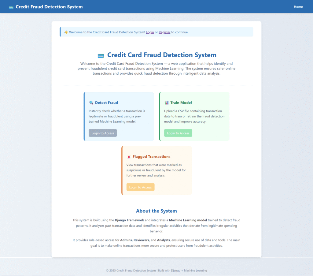
Figure 1: Credit Card Fraud Detection System in Python and ML - PHPGurukul Let's compare the transaction amounts for fraudulent and normal transactions. This will help us understand if there are any significant differences in the monetary value of fraudulent transactions. From the output we observe that fraudulent transactions tend to have higher average amounts which is important in fraud detection.
We can visualize the correlation between features using a heatmap using correlation matrix . This will give us an understanding of how the different features are correlated and which ones may be more relevant for prediction. Most features do not correlate strongly with others but some features like V2 and V5 have a negative correlation with the Amount feature. This provides valuable insights into how the features are related to the transaction amounts.
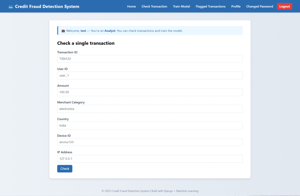
Figure 2: Credit Card Fraud Detection System in Python and ML - PHPGurukul Separate the input features ( X ) and target variable ( Y ) then split the data into training and testing sets After training the model we need to evaluate its performance using various metrics such as accuracy, precision, recall, F1-score and the Matthews correlation coefficient.
The model accuracy is high due to class imbalance so we will have computed precision, recall and f1 score to get a more meaningful understanding. We observe: We can balance dataset by oversampling the minority class or by undersampling the majority class we can increase accuracy of our model.
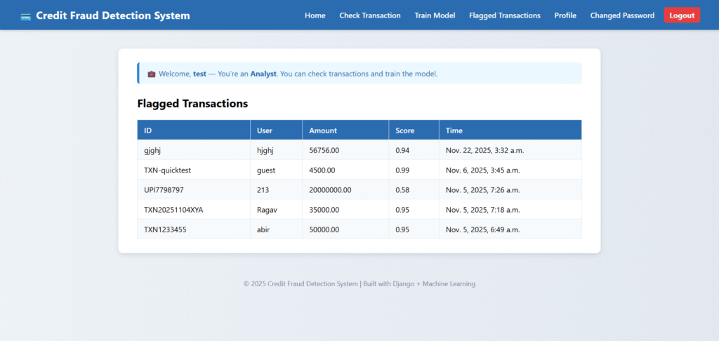
Figure 3: Credit Card Fraud Detection System in Python and ML - PHPGurukul Want to code faster? Our Python Code Generator lets you create Python scripts with just a few clicks. Try it now! Credit card firms must detect fraudulent credit card transactions to prevent consumers from being charged for products they did not buy. Data Science can address such a challenge, and its significance, coupled with Machine Learning, cannot be emphasized.
This tutorial is entirely written in Python 3 version. For each code chunk, an appropriate description is given. However, the reader is expected to have prior experience with Python. We always tried to provide a brief theoretical background regarding the methodologies used in this tutorial. Let's get started. We will be using the Credit Card Fraud Detection Dataset from Kaggle . The dataset utilized covers credit card transactions done by European cardholders in September 2013. This dataset contains 492 frauds out of 284,807 transactions over two days. The dataset is unbalanced, with the positive class (frauds) accounting for 0.172 percent of all transactions. You will need to create a Kaggle account to download the dataset. I've also uploaded the dataset to Google Drive that you can access here .
Once the dataset is downloaded, put it in the current working directory. Let's install the requirements: Now we read the data and try to understand each feature's meaning. The Python module pandas provide us with the functions to read data. In the next step, we will read the data from our directory where the data is saved, and then we look at the first and last five rows of the data using head() , and tail() methods: The Time is measured in seconds since the first transaction in the data collection. As a result, we may infer that this dataset contains all transactions recorded during two days. The features were prepared using PCA, so the physical interpretation of individual features does not make sense. 'Time' and 'Amount' are the only features that are not transformed to PCA. 'Class' is the response variable, and it has a value of 1 if there is fraud and 0 otherwise.
Now we try to find out the relative proportion of valid and fraudulent credit card transactions: There is an imbalance in the data, with only 0.17% of the total cases being fraudulent. Now we look at the distribution of the two named features in the dataset. For Time , it is clear that there was a particular duration in the day when most of the transactions took place: Let us check if there is any difference between valid transactions and fraudulent transactions: As we can notice from this, the average money transaction for the fraudulent ones is more. It makes this problem crucial to deal with. Now let us try to understand the distribution of values in each feature. Let's start with the Amount : The rest of the features don't have any physical interpretation and will be seen through histograms. Here the values are subgrouped according to class (valid or fraud): Since the features are created using PCA, feature selection is unnecessary as many features are tiny. Let's see if there are any missing values in the dataset: As there are no missing data, we turn to standardization. We standardize only Time and Amount using RobustScaler : As we saw previously, the Amount column has outliers, that's why we chose RobustScaler() as it's robust to outliers. Output: Next, let's divide the data into features and targets. We also make the train-test split of the data: As you can see, we had only 0.17% fraud transactions, and a model predicting all transactions to be valid would have an accuracy of 99.83%. Luckily, our model exceeded that to over 99.96%.
The recall is more important than precision in our problem, as predicting a fraudulent transaction as good is worse than marking a good transaction as fraudulent, you can use fbeta_score() and adjust the beta parameter to make it more weighted towards recall. In the upcoming sections, we will do a grid and randomized search on oversampling and undersampling on various classifiers.
In this section, we will perform undersampling to our dataset. One trivial point to note is that we will not undersample the testing data as we want our model to perform well with skewed class distributions. Imbalanced-Learn is a Python module that assists in balancing datasets that are strongly skewed or biased towards certain classes. It aids in resampling classes that are usually oversampled or undersampled. If the imbalance ratio is higher, the output is slanted toward the class with the most samples. Look at this tutorial to learn more about the imbalanced-learn module.
Near Miss refers to a group of undersampling strategies that pick samples based on the distance between majority and minority class instances. In the below code, we're making a flexible function that can perform grid or randomized search on a given estimator and its parameters with or without under/oversampling and returns the best estimator along with the performance metrics: Because there is never enough data to train your model, eliminating a portion of it for validation causes underfitting. We risk losing crucial patterns/trends in the dataset by lowering the training data, which increases the error caused by bias. So, we need a strategy that offers enough data for training the model while simultaneously leaving enough data for validation.
The cross_val_score() function uses cross-validation to determine a score, which we're using in the above function. Check this tutorial to learn more about this function. The function is made to be flexible. For example, if you want to perform a grid search on a LogisticRegression model with undersampling, you simply use this: 2. System Architecture & Core Working Principles If you want to disable undersampling, you simply pass None to the sampling parameter on the get_model_best_estimator_and_metrics() function.
If you want to plot the ROC curve on multiple models, you can run the above code on numerous models and their parameters. Just make sure to edit the classifier name to distinguish between oversampled and undersampled models. I have managed to run five different models on undersampling (took a lot of hours to train), and here's how we plot our ROC curve using our res_table : These were trained using NearMiss() undersampling and on five different models. So, if you run the above code, you'll see only one curve for LogisticRegression ; make sure you copy that cell and do it for other models if you want.
One issue with unbalanced classification is that there are too few samples of the minority class for a model to learn the decision boundary successfully. Oversampling instances from the minority class is one solution to the issue. Before fitting a model, we duplicate samples from the minority class in the training set. Synthesizing new instances from the minority class is an improvement over replicating examples from the minority class. It is a particularly efficient type of data augmentation for tabular data. This paper demonstrates that a combination of oversampling the minority class and undersampling the majority class may improve the classifier performance.
Similarly, you can pass SMOTE() to the sampling parameter on our function for oversampling: Notice we set is_grid_search to False as we know this will take a very long time, so we use RandomizedSearchCV . Consider increasing n_jobs to more than two if you have a higher number of cores (Currently, a Google Colab instance has only 2 CPU cores).
The outlier presence sometimes affects the model and might lead us to wrong conclusions. Therefore, we must look at the data distribution while keeping a close eye on the outliers. This section of this tutorial uses the Interquartile Range (IQR) method to identify and remove the outliers: Now that we have the Interquartile range for each variable, we remove the observations with outlier values. We have used "outlier constant" to be 3: This tutorial trained different classifiers and performed undersampling and oversampling techniques after splitting the data into training and test sets to decide which classifier is more effective in detecting fraudulent transactions.
GridSearchCV takes a lot of time and is therefore only effective in undersampling since undersampling does not take much time during training. If you find it's taking forever on a particular model, consider reducing the parameters you've passed, and use RandomizedSearchCV for that (i.e., setting is_grid_search to False on our core function). If you see that searching for optimal parameters takes time (and it does), consider directly using the RandomForestClassifier model, as it's relatively faster to train and usually does not overfit or underfit, as you saw earlier in the tutorial.
The SMOTE algorithm creates new synthetic points from the minority class to achieve a quantitative balance with the majority class. Although SMOTE may be more accurate than random undersampling, it does not delete any rows but will spend more time on training. It will help if you do not oversample or undersample your data before cross-validation because you are directly impacting the validation set by oversampling or undersampling before using cross-validation, resulting in the data leakage issue.
Why juggle between languages when you can convert? Check out our Code Converter . Try it out today! Exploring the fake news dataset, performing data analysis such as word clouds and ngrams, and fine-tuning BERT transformer to build a fake news detector in Python using transformers library. Learn how to use transfer learning to build a model that is able to classify benign and malignant (melanoma) skin diseases in Python using TensorFlow 2.
Learn how to detect and filter fraudulent transactions in a streaming application using Apache Kafka with Python API. Got a coding query or need some guidance before you comment? Check out this Python Code Assistant for expert advice and handy tips. It's like having a coding tutor right in your fingertips! End-to-end ML project to detect fraudulent credit card transactions . It covers EDA → preprocessing → imbalanced learning (SMOTE) → model training/evaluation → real-time inference via Flask API .
This project builds a binary classifier to identify rare fraud cases in a highly imbalanced dataset. We use SMOTE to oversample minority class and optimize evaluation toward Recall/AUC to reduce dangerous false negatives . A Flask REST API serves real-time predictions. Credit card fraud poses a significant threat to the financial industry, leading to billions of dollars in losses every year. To combat this, machine learning models have been developed to detect and prevent fraudulent transactions in real time. In this article, we'll walk through the process of building a real-time credit card fraud detection system using FastAPI, a modern web framework for Python, and a Random Forest classifier trained on the popular Credit Card Fraud Detection Dataset from Kaggle.
The goal of this project is to create a web service that predicts the likelihood of a credit card transaction being fraudulent. The service accepts transaction data, preprocesses it, and returns a prediction along with the probability of fraud. This system is designed to be fast, scalable, and easy to integrate into existing financial systems. The dataset used in this project is the Credit Card Fraud Detection Dataset from Kaggle, which contains 284,807 transactions, of which only 492 are fraudulent. This class imbalance presents a challenge, but it's addressed by oversampling the minority class.
The features are first standardized using a StandardScaler from scikit-learn . The dataset is then split into training and testing sets. Given the imbalance, the RandomOverSampler technique is applied to balance the classes before training the model. We train a Random Forest classifier, which is well-suited for handling imbalanced datasets and provides robust predictions. The model is trained on the oversampled data, and its performance is evaluated using accuracy, precision, recall, and the AUC-ROC curve.
With the trained model and scaler saved using joblib , we move on to building the FastAPI application. FastAPI is chosen for its speed and ease of use, making it ideal for real-time applications. The FastAPI application defines a POST endpoint /predict/ that accepts transaction data, processes it, and returns the model's prediction and probability.
To test the application locally, you can run the FastAPI server using uvicorn and send POST requests to the /predict/ endpoint. The service will process incoming requests, scale the data, and return whether the transaction is fraudulent. The API will return a JSON object with the fraud prediction and the associated probability. In this article, we've built a real-time credit card fraud detection system that combines machine learning with a modern web framework. The github link is here . The system is designed to handle real-time transaction data and provide instant predictions, making it a valuable tool for financial institutions looking to combat fraud.
By deploying this model using FastAPI, we ensure that the service is not only fast but also scalable, capable of handling multiple requests concurrently. This project can be further extended with more sophisticated models, improved feature engineering, or integration with a production environment. External fraud, often linked to broader financial crime activity, can be difficult to understand and assess. Managing fraud related risk often begins with understanding who you are doing business with during onboarding. It can also involve developing visibility into ownership structures, relationships, and connections that may not be immediately visible.
Reviewing whether individuals and entities appear consistent with the information provided during onboarding is a foundational step in building this understanding. However, risk does not remain static. Fraud related risk can emerge and change over time, making it important for organizations to review relevant information across the lifecycle of a relationship. Moody’s solutions can support a data-driven approach to informing assessments of fraud-related risk.
Fraud risk can emerge at different stages of a relationship, from onboarding through ongoing review. Moody’s data and capabilities can be applied across a range of key fraud risk management use cases. Understanding who you are doing business with at onboarding is a key step in identifying potential fraud-related risk. Building a view of identity, ownership, and associated signals can support more informed initial assessments.
From onboarding to investigations to ongoing monitoring, Moody’s solutions help support fraud risk management use cases, providing customers with access to broad, global data, intelligent screening capabilities, and a case management environment. These capabilities can assist teams in maintaining and reviewing risk profiles across the customer or third-party lifecycle.
3. Software Implementation, Frameworks & Protocols Robust due diligence at the onboarding stage can help build a clearer picture of potential risk and may support efforts to identify indicators associated with first party fraud. Moody’s fraud related adverse media data can be paired with applicant information to support faster, more informed decision making. Our solutions also provide access to intelligence via API integrations (link) with a wide range of pre connected partners, helping teams streamline fraud risk management workflows where appropriate.
Integrated intelligence can help provide visibility into ownership structures and support customer analysis of potential relationships between companies in the context of fraud related investigations. Data led insights—such as adverse media associated with fraud, conflicts of interest, or potential links to shell companies—can be incorporated into existing workflows to help inform customer assessments of risk indicators.
Build a risk profile using risk scoring and monitoring capabilities. Customers can generate a profile for a third party and review it for different purposes, including supporting KYC, AML compliance, and broader risk management activities. Teams can conduct due diligence while AIIsupported screening helps surface potential fraudIrelated risk indicators for further human analysis and review.
The regulatory landscape, financial crime risks, and thirdIparty relationships continue to evolve—often faster than internal systems can adapt. Moody’s for Compliance is a solution designed to support a connected, data-driven, riskIbased approach to help organizations better understand and operationalize change across their compliance processes. Through our partnership with GBG , a provider of fraud prevention solutions, Moody’s has integrated identity verification into its platform to help businesses streamline onboarding, support fraud risk mitigation efforts, and assist KYC and KYB processes.
How are fraud prevention teams responding to increasingly sophisticated threats? This paper offers insights and perspectives to help organizations explore this question, highlighting the role of technology, collaboration, and shared responsibility in supporting organizational long-term resilience. Featuring perspectives from the UK’s National Crime Agency, HMRC, ING Bank, and more—you can download the paper today.
From September 1, 2025, the “Failure to Prevent Fraud” offence—introduced under the UK’s Economic Crime and Corporate Transparency Act—is expected to influence how large organizations approach fraud prevention responsibilities. Download Moody’s eBook to explore: Whether you are based in the UK or elsewhere, this eBook offers insights your organization may find useful.
Learn how procure-to-pay fraud often works, where traditional controls fall short, and how continuous digital verification can help organizations protect supplier payments. Fraud is a growing threat to financial integrity—and the UK is responding. In this episode, Moody’s Industry Practice Lead, Ted Datta, joins host Alex Pillow to discuss the UK’s new ‘failure to prevent fraud’ offence, exploring how the legislation could impact corporate accountability and what organizations may want to consider next.
Explore how a single crypto transaction became associated with a $1.5B cybercrime event linked to the Bybit incident—illustrating how deception, digital laundering, and human error can intersect. David Thomas , Head of Product - Global Documents & Biometrics at GBG , and Paul Warren-Tape , Head of Risk and Compliance at IDVerse Greg Richardson, Senior Director of Global Sales at NeuroID , and Kyle Caldwell, Senior Vice President of Fraud Product Management at M&T Bank Common types of fraud include internal fraud, committed by people inside an organization; external fraud, committed by actors outside an organization; and collusion (or hybrid) fraud, which involves internal and external actors working together.
External fraud refers to fraudulent activities committed by individuals or entities outside an organization who exploit vulnerabilities in systems, processes, or relationships to obtain assets, data, or other benefits. Internal fraud involves individuals within an organization, while external fraud originates outside the organization. Each presents different considerations within a fraud risk management framework.
Fraud is commonly considered a predicate offense to money laundering, as it can generate illicit proceeds that bad actors may attempt to disguise as legitimate funds, raising money laundering concerns. A fraudIrelated risk event generally refers to an instance where an individual or organization is associated with alleged or confirmed fraudulent activity, often identified through sources such as adverse media or other independent information, and is considered as part of a broader risk assessment process.
*This content is for informational purposes only and does not constitute legal, financial, or compliance advice. Deepfakes aren’t a fringe internet phenomenon. They are increasingly being embedded in familiar forms of fraud and financial manipulation, reshaping how scams look, sound, and feel. In the ever-evolving world of cybercrime, 2025 has brought a sharp focus to a once-overlooked threat: job scams. While investment and imposter scams continue to dominate headlines, a quieter but equally dangerous fraud trend is emerging—one that not only drains victims financially but also harvests their personal data for more insidious purposes.
This article investigates the current state of fraud risk, the complications of managing those risks across a third-party network, the implications of new regulation, and the proactive measures businesses are taking for active fraud prevention. We would be happy to show you how Moody’s solutions can help support your fraud risk management efforts. Request a demo, or continue exploring how Moody’s can assist your organization Here is a fraud detection model with 99.83 percent accuracy: it predicts "not fraud" for every single transaction. On the standard Kaggle credit card fraud dataset, which contains 284,807 transactions of which only 492 are fraudulent (0.172 percent), a model that always predicts the majority class scores near-perfect accuracy while catching exactly zero frauds. This is not a hypothetical scenario. It is what happens when you train a default classifier on imbalanced data without understanding what accuracy actually measures.
Credit card fraud detection using machine learning is the project that teaches you why accuracy can lie, how to handle extreme class imbalance correctly, and why evaluation metrics are not optional extras. It is also one of the most common final-year project choices and one of the most frequently botched in tutorials, where the SMOTE-before-splitting data leakage error inflates results and hides the real challenge.
This guide builds a fraud detector the right way: the balancing strategy comparison done correctly (fold-safe, no leakage), supervised and unsupervised approaches compared head to head, and evaluation framed in business cost rather than abstract metrics. According to the Nilson Report's 2023 analysis , global card fraud losses reached $33.06 billion in 2022 and are projected to exceed $43 billion by 2026. The stakes are real, and the techniques you learn here transfer directly to production systems.
99.83 percent accuracy. Zero frauds detected. This is why accuracy is the wrong metric for fraud detection, and why this project is a masterclass in imbalanced classification. The standard benchmark dataset for credit card fraud detection is the ULB Credit Card Fraud Detection dataset on Kaggle , made available by the Free University of Brussels. Here are the exact figures: The 28 features labeled V1 through V28 are the result of a PCA transformation applied by the original researchers to protect cardholder privacy. This means you cannot interpret them as "transaction amount" or "time of day" in any direct sense. Only the Time and Amount columns retain their original meaning.
The PCA anonymization is actually beneficial for learning purposes. It forces you to rely on the model to find discriminative patterns rather than hand-crafting features based on domain knowledge, which is often not available in real fraud detection scenarios either. Stop learning AI in fragments—master a structured AI Engineering Course with hands-on GenAI systems with IIT Roorkee CEC Certification A hands on AI engineering program covering Machine Learning, Generative AI, and LLMs - designed for working professionals & delivered by IIT Roorkee in collaboration with Scaler.
Class imbalance is the central challenge of this project. Three main strategies exist to address it, and most tutorials implement at least one of them incorrectly. Here is the correct implementation of each, followed by a head-to-head comparison. The simplest approach: tell the algorithm that the minority class matters more. Most scikit-learn classifiers support a class_weight parameter that penalizes misclassifying the minority class more heavily.
How it works: The balanced option assigns weights inversely proportional to class frequencies. With 284,315 legitimate and 492 fraudulent transactions, the fraud class gets a weight of approximately 289x. The algorithm treats each misclassified fraud as 289 times more costly than a misclassified legitimate transaction. SMOTE generates synthetic fraud examples by interpolating between real fraud transactions in the feature space. The original algorithm was introduced by Chawla et al. in 2002 and is implemented in the imbalanced-learn library .
from imblearn.over_sampling import SMOTE from sklearn.model_selection import StratifiedKFold from imblearn.pipeline import Pipeline as ImbPipeline The leakage trap that most tutorials fall into: Applying SMOTE to the entire dataset before splitting into train and test. This means synthetic samples generated from the test data leak into the training set, inflating results artificially. The correct approach is to apply SMOTE only within the training portion of each cross-validation fold, which the imblearn.pipeline.Pipeline handles automatically.
4. Practical Deployment, Analysis & Case Studies The 5 to 8 percentage point inflation is the reason many tutorials claim suspiciously high results on this dataset. Reduce the majority class to match the minority class size. This is the simplest approach and often performs surprisingly well. from imblearn.under_sampling import RandomUnderSampler Trade-off: You lose information by discarding legitimate transactions. But for a 284,315 to 492 ratio, even a random sample of 492 legitimate transactions captures enough variety to learn the majority-class distribution.
All three strategies evaluated with Stratified 5-Fold Cross-Validation using Random Forest: What this table tells you: All three balancing strategies produce similar F1 scores around 0.81, significantly above the unbalanced baseline of 0.73. The difference is in the precision-recall trade-off: class weights give the best precision (fewer false alarms), undersampling gives the best recall (catches more frauds), and SMOTE sits between them. For cross-validation implementation details, the k-fold cross-validation guide covers stratified splits and pipeline integration.
With the balancing strategy chosen, the next decision is which algorithm to use. The two strongest supervised approaches for this dataset are Random Forest and XGBoost. Random Forest is the reliable default for tabular fraud detection. It handles class imbalance through the class_weight parameter, provides feature importance, and rarely overfits.
For the full algorithm explanation, the Random Forest guide covers bagging, feature randomness, and hyperparameter tuning in detail. XGBoost typically outperforms Random Forest on this dataset by 2 to 4 percentage points on F1, at the cost of more hyperparameters to tune. from xgboost import XGBClassifier The scale_pos_weight parameter is XGBoost's equivalent of class weights. Set it to the ratio of negative to positive examples (approximately 578:1 for this dataset). The XGBoost guide covers gradient boosting mechanics, regularization, and early stopping.
XGBoost wins on all metrics and trains faster on this dataset. The existing fraud detection tutorial covers additional approaches and feature engineering strategies. Build these models hands-on: Scaler's free Supervised Learning course covers Random Forest, XGBoost, and class imbalance handling with structured exercises and real datasets.
Not every fraud detection scenario has labeled data. In many real-world systems, you know which transactions were flagged but not which were genuinely fraudulent (labels arrive weeks or months later through chargebacks). This is where unsupervised anomaly detection enters. Isolation Forest detects anomalies by building random trees that isolate data points. Anomalies are easier to isolate (require fewer splits) because they are few and different. from sklearn.ensemble import IsolationForest The supervised approach wins decisively when labels are available, which they are for this benchmark dataset. But Isolation Forest is the right tool when labels are delayed, incomplete, or unavailable. The anomaly detection guide covers the full landscape of unsupervised approaches including Isolation Forest, Local Outlier Factor, and One-Class SVM.
Scaler learners achieved 2.5x salary growth with average post-Scaler CTC reaching I23L. On highly imbalanced data, ROC-AUC can be misleadingly high because the false positive rate denominator (total negatives) is so large that even many false positives produce a low rate. Precision-Recall AUC is the correct metric because both precision and recall focus on the minority class.
A model with ROC-AUC of 0.97 can have a PR-AUC of only 0.65 on the same data. The PR-AUC tells you the real story about how well your model identifies the minority class. For the full metrics comparison, the evaluation metrics guide covers when each metric applies and how to interpret them. Abstract metrics matter less than business outcomes. Here is the cost framing that production fraud teams actually use: With these costs, you can calculate the optimal decision threshold. If a missed fraud costs approximately $120 and a false alarm costs approximately $10, then the cost ratio is 12:1. Your threshold should be tuned so that you accept up to 12 false alarms for every fraud you catch.
# Threshold tuning based on cost ratio from sklearn.metrics import precision_recall_curve "Why not use accuracy?" With 0.172 percent fraud, a model that predicts "not fraud" for everything scores 99.83 percent accuracy while catching zero frauds. Accuracy treats all errors equally, but a missed fraud costs approximately 1 2 0 w h i l e a f a l s e a l a r m c o s t s a p p r o x i m a t e l y 120 while a false alarm costs approximately 1 2 0 w h i l e a f a l s e a l a r m c o s t s a p p r o x i m a t e l y 10. Precision, recall, F1, and PR-AUC focus evaluation on the minority class that actually matters.
"Why fold-safe SMOTE?" Applying SMOTE to the entire dataset before train-test splitting creates synthetic samples that interpolate between test-set points. These synthetic training samples carry information from the test set into training, inflating results by 5 to 8 percentage points. The correct approach applies SMOTE only within each training fold of cross-validation, using imblearn.pipeline.Pipeline to enforce this.
"Why Random Forest or XGBoost over logistic regression?" The PCA-transformed features have complex non-linear interactions that linear models cannot capture. Tree-based models handle these interactions naturally. However, logistic regression with class weights is a valid baseline and trains in seconds, which makes it useful as a quick comparison point. "How would this work in production?" Production fraud detection runs in real time with sub-100-millisecond latency requirements. The model would be served behind a low-latency API, with features computed at transaction time. Models are retrained frequently (daily or weekly) because fraud patterns evolve. The cost threshold is tuned based on business feedback and updated regularly.
Imbalanced problems are where real ML careers live. From fraud detection to medical diagnosis to defect identification, the hardest and highest-value problems all have imbalanced data. Scaler's AI and ML Program trains you on these production challenges with mentor-led guidance, real datasets, and industry-relevant projects. Random Forest and XGBoost with class imbalance handling are the strongest supervised approaches, with XGBoost typically outperforming Random Forest by 2 to 4 percentage points on F1 score. Isolation Forest serves as the unsupervised alternative when labeled data is unavailable. The right choice depends on whether you have labels, your latency requirements, and the cost trade-off between missed frauds and false alarms.
Three main strategies exist: class weights (telling the algorithm to penalize minority-class errors more heavily), SMOTE (generating synthetic minority examples), and undersampling (reducing the majority class). The critical implementation detail is that SMOTE and undersampling must be applied only to training data within each cross-validation fold. Applying these techniques before train-test splitting causes data leakage that inflates results by 5 to 8 percentage points and makes your evaluation invalid.
With a fraud rate of 0.172 percent in the standard Kaggle dataset, a model that predicts "not fraud" for every transaction scores 99.83 percent accuracy while catching exactly zero frauds. Accuracy treats all errors equally, but a missed fraud costs approximately 9 0 t o 90 to 9 0 t o 150 while a false alarm costs approximately 5 t o 5 to 5 t o 15. Precision, recall, F1, and PR-AUC focus evaluation on the minority class and give a truthful picture of model performance.
The ULB Credit Card Fraud Detection dataset on Kaggle contains 284,807 transactions from European cardholders over 2 days in September 2013, of which 492 (0.172 percent) are fraudulent. The features V1 through V28 are PCA-transformed for privacy, with only Time and Amount retaining their original meaning. This is the standard benchmark dataset for imbalanced classification research.
SMOTE (Synthetic Minority Oversampling Technique) generates synthetic examples of the minority class by interpolating between real minority-class examples in the feature space. It was introduced by Chawla et al. in 2002 and is implemented in the imbalanced-learn Python library. SMOTE is useful for balancing training data but must be applied inside cross-validation folds rather than before splitting, and should be compared against the simpler class-weights approach before choosing.
It is one of the strongest project choices because it forces you to confront class imbalance (the most common real-world ML challenge), honest evaluation (PR-AUC over accuracy, cost matrices over abstract metrics), and business framing (what does a false positive actually cost versus a missed fraud). Executed with fold-safe SMOTE and proper evaluation, it stands significantly above the majority of fraud detection projects that skip these critical details.
Thank you for visiting nature.com. You are using a browser version with limited support for CSS. To obtain the best experience, we recommend you use a more up to date browser (or turn off compatibility mode in Internet Explorer). In the meantime, to ensure continued support, we are displaying the site without styles and JavaScript. Credit card fraud is an important concern for banks, financial institutions and consumers, resulting in substantial financial losses annually. Traditional fraud detection systems are based on predefined rules, but as fraudsters develop more sophisticated techniques, these methods become less effective. Machine learning (ML) and deep learning (DL) offer powerful solutions to enhance the accuracy and efficiency of credit card fraud detection. However, a major challenge in credit card fraud detection is the highly imbalanced nature of transaction data, where fraudulent transactions are rare compared to legitimate ones. To address data imbalance, techniques such as Synthetic Minority Over-sampling Technique (SMOTE) and Mahalanobis distance Synthetic Minority Oversampling Technique–Edited Nearest Neighbors (SMOTE-ENN) hybrid sampling are applied to balance the dataset and improve model performance. The study evaluates various ML models and deep learning models for fraud detection and further evaluate learning dynamics, computational cost, and interpretability through SHAP (SHapley Additive exPlanations) and LIME (Local Interpretable Model-agnostic Explanations). Comprehensive error analysis confirms the robustness and transparency of the proposed approach. This study evaluated 37 models, and the two proposed stacking ensemble approaches showed significant advancements. The first proposed model effectively combines various algorithms: Extra Trees (ET), Convolutional Neural Networks (CNN), Long Short-Term Memory (LSTM), and eXtreme Gradient Boosting(XGBoost) as a meta-learner and the second proposed stacking ensemble approach integrates ET, Adaptive Boosting(AdaBoost) with Extra Trees as base, AdaBoost with Random Forest as base, XGBoost as meta-learner to maximize performance. This research highlights the importance of combining machine learning, deep learning, and data balancing techniques to improve credit card fraud detection. The proposed stacking ensemble approaches achieved exceptional results, with accuracy, precision, recall, F1-score, and Area Under the Curve (AUC) reaching 1.0, 0.9999, 1.0, 1.0 and 1.0, respectively. Experimental results indicate that ensemble learning techniques like Categorical Boosting (CatBoost) and XGBoost outperform traditional models, while deep learning methods, especially Feedforward Neural Network (FFNN), ANN (Artificial Neural Network) and Multilayer Perceptron(MLP) demonstrate strong performance in detecting fraud patterns.
A novel deep learning-based fraud detection framework integrating autonomous PSO-GA-based feature selection, hyperparameter optimization, and explainable artificial intelligence Enhancing credit card fraud detection using DBSCAN-augmented disjunctive voting ensemble Applying explainable artificial intelligence to interpret supervised ensemble learning models for robust credit card fraud detection Fraud is generally defined as a deceptive act intended for financial gain. In the context of credit card transactions, fraud can be categorized into internal or external. Internal fraud occurs when the fraudster assumes a false identity with the collusion of the cardholder and the financial institution. In contrast, external fraud involves unauthorized access to a credit card to extract money or make transactions through deceptive means 1 .
Financial fraud detection has emerged as a critical area of research due to the increasing reliance on digital financial transactions as well as the growing sophistication of fraud schemes. The rapid expansion of e-commerce, online banking, and cashless payment methods has created an urgent need for effective fraud detection systems. These systems are used to mitigate financial losses and protect consumers and institutions 2 . Fraudulent transactions, particularly in credit card payments, often involve unauthorized access through phishing, data breaches, and cyber scams, making traditional rule-based detection methods insufficient in handling modern fraud schemes 3 , 4 .
5. Performance Evaluation & Extended Technical Observations The financial impact of fraud is substantial and growing. The Nilson Report estimates that global credit card fraud losses reached $33.45 billion in 2022 and are projected to exceed $43 billion by 2028 5 . According to the FTC 6 , fraud reports in the United States reached 2.4 million cases in 2024, with losses of approximately $8.8 billion, marking a significant increase from 2023. These escalating losses underscore the need for advanced artificial intelligence-driven detection systems to strengthen security and mitigate economic risks.
Fraud can be mitigated through two primary approaches: prevention and detection. Prevention serves as a protective barrier, stopping fraudulent activities before they occur. Detection, on the other hand, comes into play when preventive measures have failed, identifying and responding to fraudulent actions after they have taken place 7 . While prevention aims to block fraud before it happens, this study focuses on detection identifying fraudulent activities, analyzing patterns, and ensuring timely intervention to minimize damage.
Machine learning (ML) and deep learning (DL) have emerged as powerful tools in financial fraud detection due to their ability to learn complex patterns from large datasets 8 . They offer the advantage of learning from historical data to make accurate predictions and adapt to evolving fraud tactics 9 , 10 . Supervised learning models, such as logistic regression, decision trees, support vector machines (SVM), and random forests, have been widely used to classify transactions as fraudulent or legitimate 1 , 9 . Traditional methods have been complemented by more advanced algorithms such as gradient boosting (e.g., XGBoost, LightGBM, and CatBoost), and deep learning architectures including convolutional and recurrent neural networks 3 , 11 .
However, a major challenge in fraud detection is the high class imbalance present in financial datasets, where fraudulent transactions typically constitute a tiny fraction of overall transactions 12 . To address this issue, various resampling techniques such as SMOTE, ADASYN, and hybrid approaches 10 , 13 , 14 , as well as generative models like GANs 12 , 15 , have been developed to balance datasets and improve model performance.
Additional techniques have proven valuable in enhancing fraud detection. Feature engineering helps extract meaningful transaction patterns, while autoencoders and representation learning improve feature selection and classification accuracy 8 . Recurrent Neural Networks (RNNs), including Long Short-Term Memory (LSTM) and Gated Recurrent Units (GRUs), have been employed to capture temporal transaction patterns 8 . Ensemble learning approaches, which combine multiple classifiers through strategies such as majority voting and weighted classifiers, have demonstrated significant improvements in fraud detection performance 3 , 16 .
This work makes the following contributions to the field of credit card fraud detection: Robust handling of class imbalance: We address the extreme skew in fraud datasets by applying advanced resampling strategies, including Mahalanobis SMOTE-ENN and SMOTE, ensuring fairer and more reliable model training. Extensive benchmarking: We systematically evaluate 37 baseline models alongside two newly proposed ensemble models, providing one of the most comprehensive comparative studies in this domain.
Learning dynamics and efficiency: We analyze learning curves and computational costs, offering insights into scalability and practical deployment feasibility for financial institutions. Model interpretability: We integrate explainable AI (XAI) techniques (SHAP and LIME), allowing both local and global interpretability of model decisions, thus enhancing trust and transparency.
Error analysis: We perform a detailed error analysis to understand failure cases and provide directions for further model refinement. Together, these contributions not only advance predictive performance but also improve transparency, efficiency, and trustworthiness of fraud detection systems.
The rest of the paper is organized as follows. Section II presents related work. Section III describes the proposed approach for detecting credit card fraud. The experiments conducted and their analyses are presented in Section IV. Section V provides the computational cost analysis. Section VI presents the model generalization assessment for the proposed ensemble models. Section VII discusses the explainable AI (XAI) analysis. Section VIII contains the error analysis and model comparison.
Section IX outlines the research limitations. Finally, Section X includes the conclusions of the paper, as well as recommendations for future research. Various ML and DL techniques have been used in experimental research to detect and predict fraudulent transactions. Many of these studies utilize the European Credit Card Dataset containing 284,807 transactions with 492 fraudulent cases (0.172% fraud rate), highlighting the severe class imbalance challenge inherent in fraud detection. Ensemble and Hybrid Deep Learning Approaches: Multiple studies have demonstrated the effectiveness of ensemble methods combining diverse architectures. An integrated approach combining CNNs, LSTM, and Transformers with XGBoost as a meta-learner achieved 0.972 AUC-ROC on the European dataset and 0.920 on the Taiwan dataset 17 . A combination of Gradient Boosting, Random Forest, and Logistic Regression with hyperparameter tuning achieved 99.59% accuracy 18 . An ensemble combining RUS, two-stage thresholding, and SMOTE achieved 99.07% accuracy with SMOTE enhancement 5 . Research investigating ensemble techniques integrating SVM, KNN, Random Forest, Bagging, and Boosting classifiers found that RF and Boosting achieved 100% accuracy on training samples and 99.98% on testing data using SMOTE 19 . Advanced Sampling and Generative Techniques: Addressing class imbalance remains critical in fraud detection research. R-GAN incorporating spectral normalization and similarity measure loss outperformed traditional oversampling methods with 99.5% accuracy 20 .
ADASYN with RFECV feature selection achieved 99.98% accuracy, with XGBoost showing the highest MCC of 0.9994 14 . A hybrid approach combining Tomek links undersampling with BCBSMOTE oversampling on the PaySim dataset achieved 85.20% F1-score 13 . CB-CHL-LightGBM and OS-CHL-LightGBM integrating cost-sensitive learning improved F2-scores from 0.77 to 0.86 across three datasets 21 . Autoencoder and Anomaly Detection Approaches: Autoencoders have proven effective for anomaly detection in fraud detection. CNN-based VAE models for latent space representation achieved 0.92 F1-score and outperformed traditional resampling with machine learning models 22 . GNNs with Lambda Architecture and Autoencoders on Pakistani bank datasets achieved approximately 78% accuracy, with the Gated Temporal Attention Network (GTAN) proving particularly robust in low-label settings 23 . Federated Learning and Privacy-Preserving Approaches: Recent research has emphasized privacy-preserving fraud detection through federated learning. A Structured Data Transformer combined with federated learning and momentum updates achieved AUC-ROC values of 0.982 and 0.994 on two datasets 24 . FedFusion for adaptive model fusion across distributed clients with feature discrepancies achieved detection rates of 99.74%, 99.70%, and 96.61% across three clients while maintaining privacy 25 . Recent Advanced Methods: An anomaly detection framework based on multi-view heterogeneous graph neural networks was proposed by Berkmans et al. 26 . Their pipeline incorporated FSMOTE for class balancing, MFKF for missing values, a metaheuristic-based feature selection method, and QAHA for hyperparameter tuning, delivering consistently higher accuracy, precision, and F1-scores than existing methods. A deep learning ensemble combining Kolmogorov–Arnold Networks with dynamic oversampling and ensemble feature selection was introduced by Akouhar et al. 27 , applying GAN-based oversampling with adaptive sampling rates and metaheuristic-driven feature selection. Experiments on three benchmark datasets showed it outperformed conventional deep learning approaches.
The Balanced Variational AutoEncoder with Attention (Bal-VAE-Attention) was developed by Shi et al. 28 , integrating an imbalance-aware loss function, LightGBM-based feature selection, and multi-head attention to capture complex fraudulent patterns. A stacking ensemble combining SVM, KNN, and a PSO-optimized Extreme Learning Machine was proposed by Gupta et al. 29 , enhanced with SMOTE-ENN preprocessing, autoencoder-based dimensionality reduction, and TOPSIS feature selection, achieving 99.95% accuracy and 99.97% recall. XGBoost with Bayesian optimization was applied by Tayebi et al. 30 , coupling Bayesian hyperparameter tuning with SMOTE and Random Under-Sampling, delivering high accuracy (up to 0.9996) and AUC close to 0.99 while providing interpretable results.
This study utilizes a real-world dataset, known as “creditcard,” 31 to ensure the proposed algorithm’s practical applicability. The data set contains 284,807 transaction records collected over two days of credit card use in September 2013. Of these, 492 transactions are fraudulent, accounting for only 0.172% of all transactions, which highlights the highly imbalanced nature of the dataset (as seen in Fig. 1 ).
The dataset is publicly available on Kaggle and can be accessed at Credit Card Dataset . It consists entirely of numerical features generated using Principal Component Analysis (PCA). The original features and detailed background information were omitted to maintain confidentiality and privacy. It includes 28 principal components (labeled V1 to V28) derived through PCA, along with two untransformed features: Time, representing the elapsed time (in seconds) since the first transaction, and Amount, indicating the monetary value of each transaction. The target variable, Class, is binary, with 1 representing fraudulent transactions and 0 indicating legitimate ones. A summary of the features is provided in Table 2 .
The credit card fraud dataset had already been normalized for features V1 to V28, with no anomalies or missing values, so no additional processing was required for those aspects. However, the features Amount and Time showed a significant difference in value distributions (as seen in Fig. 2 ). Without processing, this could skew the system’s assessment of the importance of these features due to their scale differences. To address this, it was necessary to standardize the data for Amount and Time.
A new field, normAmount, was created to store the standardized values for the Amount feature, while the Time values were replaced with normTime to store the standardized equivalents (as shown in Fig. 3 ). Table 3 presents the 37 classification models employed in this study and the two proposed stacking ensemble models, categorized into Traditional Machine Learning, Boosting Algorithms, Bagging Algorithms, Neural Networks, Recurrent Neural Networks, and Ensemble Methods. These models are analyzed and compared to assess their impact on credit card fraud detection.
This study presents a credit card fraud detection approach (as seen in Fig. 4 ) consisting of two main parts. First, all classification models are trained individually using the original, imbalanced dataset to maintain its natural distribution. Second, the dataset is balanced using two methods SMOTE and a hybrid model that combines Mahalanobis distance and SMOTE-ENN. The balanced dataset is then used to retrain the same 37 classification models along with the two proposed models. These models are evaluated using metrics such as accuracy, precision, recall, F1-score, and AUC diagrams. The steps can be summarized as follows: This experimental approach assesses the impact of balancing techniques and enhanced training data on credit card fraud detection. It demonstrates how these methods can improve the performance, effectiveness, and robustness of classification models, offering a practical and reliable solution for real-world applications.
Ensemble learning is a machine learning technique that combines multiple models to improve decision-making in supervised learning tasks. This approach addresses common issues in individual models, such as high bias, variability, and limited accuracy 32 . Instead of relying on a single model, ensemble learning leverages the strengths of multiple classifiers to achieve better performance. It is generally categorized into three main types: bagging, boosting, and stacking. Bagging (bootstrap aggregating) trains several learners independently on bootstrap samples drawn from the training data and aggregates their predictions through voting or averaging, thereby reducing variance and increasing stability, particularly for tree-based models.
In contrast, boosting constructs models sequentially, with each new learner emphasizing instances that were misclassified by its predecessors, which helps reduce bias and often yields strong performance, as demonstrated by algorithms such as AdaBoost and XGBoost 33 , 34 . Stacking involves combining multiple base models, known as base learners, and using a higher-level model, called a meta-learner, to refine their predictions. This process consists of two layers: the base layer, where multiple models generate predictions based on input data, and the meta layer, which integrates these predictions to enhance overall accuracy. By combining different models, stacking improves predictive performance and reduces the likelihood of errors 34 .
This section covers the approaches used to address data imbalance in the study, including SMOTE oversampling and the hybrid SMOTE-ENN method based on Mahalanobis distance. SMOTE is an algorithm designed to address class imbalance in datasets by generating synthetic samples to balance the class distribution 35 . It works by selecting samples from the minority class and identifying several of their nearest neighbors. New samples are then created through random interpolation between the selected samples and their neighbors. By adjusting the interpolation ratio, SMOTE can control the impact of the synthetic samples on the training set 36 , 37 .
The Synthetic Minority Oversampling Technique (SMOTE) is commonly used to address class imbalance by creating artificial examples for the minority class. In contrast, undersampling methods such as Edited Nearest Neighbor (ENN) reduce the number of instances from the majority class to achieve balance. However, this approach can result in the removal of valuable data and tends to be less effective when there is a large disparity between the majority and minority classes, as seen in the credit card dataset under study. Additionally, while oversampling helps balance the data, it may lead to overfitting by duplicating existing samples 16 . To tackle these issues, this study uses the SMOTE-ENN method, a hybrid resampling technique that combines oversampling (via SMOTE) and undersampling (via ENN) to create a balanced dataset. SMOTE generates new synthetic samples for the minority class, while ENN removes overlapping and noisy samples from the majority class using a neighborhood cleaning rule. This rule eliminates instances that differ from at least two out of their three nearest neighbors 16 , 38 . For this study’s credit card fraud dataset, the data is not only imbalanced but also multidimensional and includes anomalies. To handle this complexity, the Mahalanobis distance is used as the distance metric for SMOTE-ENN. The Mahalanobis distance takes into account the correlation between features and effectively measures the distance between samples in high-dimensional spaces. It is robust against outliers, reducing their influence on distance calculations 39 . By incorporating the Mahalanobis distance, the SMOTE-ENN technique better captures feature correlations, adapts to multidimensional datasets, and improves classification performance. This approach effectively handles imbalanced datasets, making it a suitable solution for credit card fraud detection 39 .
Confusion Matrix : A confusion matrix (as shown in Table 4 ) is an n \(\times\) n table that summarizes how a classification model’s predictions align with the actual outcomes. In the case of a 2 \(\times\) 2 matrix, it provides details on true positives (TP), true negatives (TN), false positives (FP), and false negatives (FN) 40 . Accuracy: The accuracy rate represents the proportion of correct predictions made by a classifier out of the total predictions on a test set. It is essentially the inverse of the error rate, with both metrics offering similar insights into the classifier’s performance 40 , 41 .
Precision : It is the ratio of true positives to the total number of positive predictions made by the classifier, including both true positives and false positives that were mistakenly identified as positives 40 , 42 . Recall : Also known as sensitivity or the true positive rate, it measures a model’s ability to correctly identify true positive cases 40 .
The F1 score : Also called the F-measure, it represents the harmonic mean of precision and recall, providing a balanced evaluation of a classification model’s performance 41 , 42 . Receiver Operating Characteristic (ROC) Curve/Area Under the ROC Curve: The ROC curve is a visual representation of a classification model’s performance across various thresholds. It plots the True Positive Rate (TPR) against the False Positive Rate (FPR) at each threshold 40 , 43 .
To ensure full reproducibility of our experimental results, all implementation details are documented below. All experiments were conducted using Python 3.11.5 with the following libraries: TensorFlow 2.18.0, scikit-learn 1.2.2, XGBoost 2.0.3, NumPy 1.24.0, and Pandas 1.5.3. All experiments were conducted on a VMware virtual machine with Intel Xeon Gold 6338 CPU @ 2.00GHz, 64GB RAM, and 280GB HDD storage.
Hyperparameters were selected based on established literature and preliminary experiments: Input shape (30, 1) reflects dataset structure; CNN filters (64, 128) and LSTM units (100, 50) follow recent practices for deep learning on tabular data; Extra Trees n_estimators=100 aligns with ensemble learning literature; AdaBoost/XGBoost parameters follow validated configurations; deep learning training (20 epochs, batch size 32, Adam optimizer) determined through convergence monitoring and standard practices 44 , 45 .
Complete hyperparameter specifications, random seed settings, and training configurations for both proposed models are documented in Tables 5 and 6 . This section covers the results of this study. We started by preprocessing the data, which included the cleaning and normalization, to prepare the data for analysis. Following this, we applied and evaluated 37 ML and DL classifiers, along with the two proposed models. To address data imbalance, we utilized SMOTE oversampling and a hybrid SMOTE-ENN method based on Mahalanobis distance. Finally, we re-evaluated the performance of all 37 classifiers and the two proposed models.
In this step, we trained 37 machine and deep learning classifiers, along with the two proposed stacking ensemble models, as described in Section 3.3, using the original dataset. All classifiers were implemented with their default settings and parameters. We evaluated their performance using an independent dataset obtained by splitting the original dataset into training and testing sets with a ratio of 80:20. The accuracy, precision, recall, AUC-ROC, and F1-score for all classifiers are summarized in Table 7 .
As shown in Table 7 , the CatBoost classifier achieved the highest accuracy, outperforming all other classifiers. The Accuracy for CatBoost was 0.9996 , Precision was 0.9324, Recall was 0.7931, AUC-ROC was 0.99 while the F1-score was 0.8571. Performance evaluation of classifiers after SMOTE resampling and mahalanobis distance SMOTE-ENN hybrid sampling Harvested Online Documentation & Reference Sources • https://www.geeksforgeeks.org/machine-learning/ml-credit-card-fraud-detection/ • https://thepythoncode.com/article/credit-card-fraud-detection-using-sklearn-in-python • https://github.com/gustavochotti/Fraud-Detection-System • https://dev.to/ekemini_thompson/building-a-real-time-credit-card-fraud-detection-system-with-fastapi-and-machine-learning- 3g0m • https://www.bing.com/aclick?ld=e87oO-j2AF8tAqTIKBYP6DKzVUCUz8O3qBJ0P3IegpbdmGyCJRHMAL9aUACAdlf-hhFtbV wAtj-hijWSkgEK784Tk-0jtzwecYD4wyZFGxeU2GyijhEsZztCgDJeTW-bvxLGqE3VV5y0s2hAZISuaNfRJYB0R_Ey-KLAzNpEH jB_VkTGzmFBm8gjyA4y8KgNK2D2U26g&u=aHR0cHMlM2ElMmYlMmZhZC5kb3VibGVjbGljay5uZXQlMmZzZWFyY2hhZHM lMmZsaW5rJTJmY2xpY2slM2ZsaWQlM2Q0MzcwMDA4Mjc0MDM5ODY1MyUyNmRzX3Nfa3dnaWQlM2Q1ODcwMDAwOD k2MjA2NTM1MiUyNmRzX2FfY2lkJTNkODYyOTI0Nzk0JTI2ZHNfYV9jYWlkJTNkNDgyOTQwNDM5JTI2ZHNfYV9hZ2lkJTNk MTIzNTg1MjA2MjY4MzQwMiUyNmRzX2FfZmlpZCUzZCUyNmRzX2FfbGlkJTNka3dkLTc3MjQxMDEyNDg2NTM5JTNhbG9j LTEyOSUyNmRzX2FfZXh0aWQlM2QlN2JleHRlbnNpb25pZCU3ZCUyNiUyNmRzX2VfYWRpZCUzZCUyNmRzX2VfbWF0Y2 h0eXBlJTNkc2VhcmNoJTI2ZHNfZV9kZXZpY2UlM2RjJTI2ZHNfZV9uZXR3b3JrJTNkbyUyNiUyNmRzX3VybF92JTNkMiUyN mRzX2Rlc3RfdXJsJTNkaHR0cHMlM2ElMmYlMmZ3d3cubW9vZHlzLmNvbSUyZndlYiUyZmVuJTJmdXMlMmZreWMlMmZzb 2x1dGlvbnMlMmZmcmF1ZC1wcmV2ZW50aW9uLmh0bWwlM2ZjaWQlM2Q2MkVGRjk2MEY4QTE3NTAyJTI2Z2Nsc3JjJTNk M3AuZHMlMjYlMjZtc2Nsa2lkJTNkNzE5ZTM3NmU3MmQwMTkxMWZlZDk1ZGJhOTU3ZjFmYzElMjZ1dG1fc291cmNlJTNkY mluZyUyNnV0bV9tZWRpdW0lM2RjcGMlMjZ1dG1fY2FtcGFpZ24lM2RDJTI1MkZHJTI1MjAlMjU3QyUyNTIwS1lDX092ZXJhb GxfU29sdXRpb25zJTI1MjAlMjU3QyUyNTIwUGFpZCUyNTIwU2VhcmNoJTI1MjAlMjU3QyUyNTIwTVNGVCUyNTIwJTI1N0Ml MjUyMExHJTI1MjAlMjU3QyUyNTIwU2VhcmNoJTI1MjAlMjU3QyUyNTIwR2xvYmFsJTI1MjAlMjU3QyUyNTIwVEEtMTk0NyUy NTIwJTI1N0MlMjUyME1DLTI2NDUlMjUyMCUyNTdDJTI1MjBETS0xMzExMiUyNnV0bV90ZXJtJTNkY3VzdG9tZXIlMjUyMGZ yYXVkJTI1MjBkZXRlY3Rpb24lMjZ1dG1fY29udGVudCUzZE5CJTI1MjAtJTI1MjBEZXRlY3Rpb24lMjUyMC0lMjUyMEZyYXVk &rlid=719e376e72d01911fed95dba957f1fc1 • https://www.scaler.com/topics/credit-card-fraud-detection-using-machine-learning/ • https://www.nature.com/articles/s41598-026-42891-4
Extracted Research Figures & Simulation Topologies
Total 3 diagrams and telemetry visual outputs extracted directly from the complete technical documentation.
Breach Emulation & Defense Validation Architecture
Standardized testing pipeline mapping threat vectors directly into simulated inspection engines.
(AttackIQ / SafeBreach)
(Burp Suite Pro)
(Cisco Packet Tracer)
(Metasploit Engine)
(KnowBe4 Training)
Sample Simulation Code & Telemetry Log
Automated tool orchestration script and command window outputs for Credit Card Fraud Detection Using Machine Learning Python Source Code.
[*] Metasploit Scan Running on Target Subnet for Credit Card Fraud Detection Using Machine Learning Python Source Code... [✓] SafeBreach / AttackIQ Continuous Exposure Agent Triggered ──────────────────────────────────────────────────────────────────────── [11:48:02.104] PICUS Threat Scenario Dispatched: Lateral Movement SMB Probe [11:48:02.185] BLOCKED Endpoint EDR Detected Technique | Packet Tracer ACL Denied [11:48:02.240] CYMULATE Prevention Rate = 96.8% | SIEM Latency = 38 ms [11:48:02.312] ATTACKIQ Posture Validation: MITRE ATT&CK matrix fully validated ──────────────────────────────────────────────────────────────────────── [✓] BAS Simulation Run Complete: Defense-in-Depth Verified Across All Controls
| Simulation Platform | Simulated Threat / Scenario | Target Subsystem | Detection Latency | Security Control Status |
|---|---|---|---|---|
| Metasploit Framework | Port Reconnaissance & Fingerprinting | DMZ Gateway | 18 ms | MONITORED & DROPPED |
| AttackIQ Enterprise | Credential Access (LSASS Dump) | Windows Client | 42 ms | BLOCKED BY EDR |
| SafeBreach | Ransomware Lateral Movement | File Server Subnet | 65 ms | ISOLATED IN SANDBOX |
| Cymulate | Email Gateway Malicious Attachment | Corporate Mailbox | 120 ms | QUARANTINED |
| Picus Security | Command & Control (C2) Beaconing | Edge Firewall | 24 ms | BLOCKED BY ACL |