Complete Technical Paper Content — Industrial Control System Anomaly Detection Using Deep Learning
Overview & System Context
Industrial Control System Anomaly Detection Using Deep Learning: Comprehensive Web-Sourced Technical Investigation Exhaustive Research Dossier · Pure Web-Scraped Content: ~9029 Words · Real Software Screenshots: 3 1. Executive Overview & Technical Background In data analysis, anomaly detection (also referred to as outlier detection and sometimes as novelty detection) is generally understood to be the identification of rare items, events or observations which deviate significantly from the majority of the data and do not conform to a well defined notion of normal behavior. Such examples may arouse suspicions of being generated by a different mechanism, or appear inconsistent with the remainder of that set of data. Anomaly detection finds application in many domains including cybersecurity, medicine, machine vision, statistics, neuroscience, law enforcement and financial fraud to name only a few. Anomalies were initially searched for clear rejection or omission from the data to aid statistical analysis, for example to compute the mean or standard deviation. They were also removed to better predictions from models such as linear regression, and more recently their removal aids the performance of machine learning algorithms.
However, in many applications anomalies themselves are of interest and are the observations most desirous in the entire data set, which need to be identified and separated from noise or irrelevant outliers. Three broad categories of anomaly detection techniques exist: Supervised anomaly detection techniques require a data set that has been labeled as "normal" and "abnormal" and involves training a classifier. However, this approach is rarely used in anomaly detection due to the general unavailability of labelled data and the inherent unbalanced nature of the classes. Semi-supervised anomaly detection techniques assume that some portion of the data is labelled. This may be any combination of the normal or anomalous data, but more often than not, the techniques construct a model representing normal behavior from a given normal training data set, and then test the likelihood of a test instance to be generated by the model. Unsupervised anomaly detection techniques assume the data is unlabelled and are by far the most commonly used due to their wider and relevant application.
A point anomaly is an individual observation that is considered anomalous relative to the rest of the data e.g., an unusually large transaction may be anomalous when compared with the other transactions in a dataset. A contextual anomaly, also called a conditional anomaly, is anomalous only within a particular context. An observation may therefore be normal under one set of circumstances but anomalous under another e.g., a particular temperature may be normal in summer but unusual in winter. Context may be temporal, spatial, demographic, or otherwise defined by the application. A collective anomaly is a related collection of observations that is anomalous as a whole, even when its individual observations are not anomalous by themselves e.g., an unusual subsequence in a time series or an unexpected pattern of activity in a computer network. The appropriate category depends partly on the structure of the data. Point-anomaly methods may be sufficient for independent observations, whereas time series, spatial data, sequences, and graphs often require contextual or collective relationships to be modelled explicitly.
The Subspace Outlier Degree (SOD) identifies attributes where a sample is normal, and attributes in which the sample deviates from the expected. Correlation Outlier Probabilities (COP) compute an error vector of how a sample point deviates from an expected location, which can be interpreted as a counterfactual explanation: the sample would be normal if it were moved to that location.
Figure 1: AI anomaly detection industrial inspection | 2M Technology Fault detection, isolation, and recovery (FDIR) is a subfield of control engineering which concerns itself with monitoring a system, identifying when a fault has occurred, and pinpointing the type of fault and its location. Two approaches can be distinguished: A direct pattern recognition of sensor readings that indicate a fault and an analysis of the discrepancy between the sensor readings and expected values, derived from some model. In the latter case, it is typical that a fault is said to be detected if the discrepancy or residual goes above a certain threshold. It is then the task of fault isolation to categorize the type of fault and its location in the machinery. Fault detection and isolation (FDI) techniques can be broadly classified into two categories. These include model-based FDI and signal processing based FDI.
In model-based FDI techniques some model of the system is used to decide about the occurrence of fault. The system model may be mathematical or knowledge based. Some of the model-based FDI techniques include observer-based approach, parity-space approach, and parameter identification based methods. There is another trend of model-based FDI schemes, which is called set-membership methods. These methods guarantee the detection of fault under certain conditions. The main difference is that instead of finding the most likely model, these techniques omit the models, which are not compatible with data. The example shown in the figure on the right illustrates a model-based FDI technique for an aircraft elevator reactive controller through the use of a truth table and a state chart. The truth table defines how the controller reacts to detected faults, and the state chart defines how the controller switches between the different modes of operation (passive, active, standby, off, and isolated) of each actuator. For example, if a fault is detected in hydraulic system 1, then the truth table sends an event to the state chart that the left inner actuator should be turned off. One of the benefits of this model-based FDI technique is that this reactive controller can also be connected to a continuous-time model of the actuator hydraulics, allowing the study of switching transients.
Condition-based maintenance Planned preventive maintenance Preventive maintenance Corrective maintenance (does not use diagnostics) Integrated vehicle health management In fault detection and diagnosis, mathematical classification models which in fact belong to supervised learning methods, are trained on the training set of a labeled dataset to accurately identify the redundancies, faults and anomalous samples. During the past decades, there are different classification and preprocessing models that have been developed and proposed in this research area. K-nearest-neighbors algorithm (kNN) is one of the oldest techniques which has been used to solve fault detection and diagnosis problems. Despite the simple logic that this instance-based algorithm has, there are some problems with large dimensionality and processing time when it is used on large datasets. Since kNN is not able to automatically extract the features to overcome the curse of dimensionality, so often some data preprocessing techniques like Principal component analysis(PCA), Linear discriminant analysis(LDA) or Canonical correlation analysis(CCA) accompany it to reach a better performance. In many industrial cases, the effectiveness of kNN has been compared with other methods, specially with more complex classification models such as Support Vector Machines (SVMs), which is widely used in this field. Thanks to their appropriate nonlinear mapping using kernel methods, SVMs have an impressive performance in generalization, even with small training data. However, general SVMs do not have automatic feature extraction themselves and just like kNN, are often coupled with a data pre-processing technique. Another drawback of SVMs is that their performance is highly sensitive to the initial parameters, particularly to the kernel methods, so in each signal dataset, a parameter tuning process is required to be conducted first. Therefore, the low speed of the training phase is a limitation of SVMs when it comes to its usage in fault detection and diagnosis cases.
Figure 2: AI-Driven Anomaly Detection: Elevating Precision and Quality Control in ... Artificial Neural Networks (ANNs) are among the most mature and widely used mathematical classification algorithms in fault detection and diagnosis. ANNs are well known for their efficient self-learning capabilities of the complex relations (which generally exist inherently in fault detection and diagnosis problems) and are easy to operate. Another advantage of ANNs is that they perform automatic feature extraction by allocating negligible weights to the irrelevant features, helping the system to avoid dealing with another feature extractor. However, ANNs tend to over-fit the training set, which will have consequences of having poor validation accuracy on the validation set. Hence, often, some regularization terms and prior knowledge are added to the ANN model to avoid over-fitting and achieve higher performance. Moreover, properly determining the size of the hidden layer needs an exhaustive parameter tuning, to avoid poor approximation and generalization capabilities. In general, different SVMs and ANNs models (i.e. Back-Propagation Neural Networks and Multi-Layer Perceptron) have shown successful performances in the fault detection and diagnosis in industries such as gearbox, machinery parts (i.e. mechanical bearings), compressors, wind and gas turbines and steel plates.
With the research advances in ANNs and the advent of deep learning algorithms using deep and complex layers, novel classification models have been developed to cope with fault detection and diagnosis. Most of the shallow learning models extract a few feature values from signals, causing a dimensionality reduction from the original signal. By using Convolutional neural networks, the continuous wavelet transform scalogram can be directly classified to normal and faulty classes. Such a technique avoids omitting any important fault message and results in a better performance of fault detection and diagnosis. In addition, by transforming signals to image constructions, 2D Convolutional neural networks can be implemented to identify faulty signals from vibration image features. Deep belief networks, Restricted Boltzmann machines and Autoencoders are other deep neural networks architectures which have been successfully used in this field of research. In comparison to traditional machine learning, due to their deep architecture, deep learning models are able to learn more complex structures from datasets, however, they need larger samples and longer processing time to achieve higher accuracy.
Switch-off of a faulty equipment Switch-over from a faulty equipment to a redundant equipment Change of state of the complete system into a Safe Mode with limited functionalities Multi-agent reinforcement learning (MARL) is a sub-field of reinforcement learning. It focuses on studying the behavior of multiple learning agents that coexist in a shared environment. Each agent is motivated by its own rewards, and does actions to advance its own interests; in some environments these interests are opposed to the interests of other agents, resulting in complex group dynamics. Multi-agent reinforcement learning is closely related to game theory and especially repeated games, as well as multi-agent systems. Its study combines the pursuit of finding ideal algorithms that maximize rewards with a more sociological set of concepts. While research in single-agent reinforcement learning is concerned with finding the algorithm that gets the biggest number of points for one agent, research in multi-agent reinforcement learning evaluates and quantifies social metrics, such as cooperation, reciprocity, equity, social influence, language and discrimination.
Figure 3: Industrial AI - Arnest Innovative Solutions A set S {\displaystyle S} of environment states. One set A i {\displaystyle {\mathcal {A}}_{i}} of actions for each of the agents i ∈ I = { 1 , … , N } {\displaystyle i\in I=\{1,\dots ,N\}} . P a → ( s , s ′ ) = Pr ( s t + 1 = s ′ I s t = s , a → t = a → ) {\displaystyle P_{\vec {a}}(s,s')=\Pr(s_{t+1}=s'\mid s_{t}=s,{\vec {a}}_{t}={\vec {a}})} is the probability of transition (at time t {\displaystyle t} ) from state s {\displaystyle s} to state s ′ {\displaystyle s'} under joint action a → {\displaystyle {\vec {a}}} .
R → a → ( s , s ′ ) {\displaystyle {\vec {R}}_{\vec {a}}(s,s')} is the immediate joint reward after the transition from s {\displaystyle s} to s ′ {\displaystyle s'} with joint action a → {\displaystyle {\vec {a}}} . In settings with perfect information, such as the games of chess and Go, the MDP would be fully observable. In settings with imperfect information, especially in real-world applications like self-driving cars, each agent would access an observation that only has part of the information about the current state. In the partially observable setting, the core model is the partially observable stochastic game in the general case, and the decentralized POMDP in the cooperative case.
In pure competition settings, the agents' rewards are exactly opposite to each other, and therefore they are playing against each other. Pure cooperation settings are the other extreme, in which agents get the exact same rewards, and therefore they are playing with each other. Mixed-sum settings cover all the games that combine elements of both cooperation and competition.
Most real-world scenarios involving multiple agents have elements of both cooperation and competition. For example, when multiple self-driving cars are planning their respective paths, each of them has interests that are diverging but not exclusive: Each car is minimizing the amount of time it's taking to reach its destination, but all cars have the shared interest of avoiding a traffic collision. Zero-sum settings with three or more agents often exhibit similar properties to mixed-sum settings, since each pair of agents might have a non-zero utility sum between them. Mixed-sum settings can be explored using classic matrix games such as prisoner's dilemma, more complex sequential social dilemmas, and recreational games such as Among Us, Diplomacy and StarCraft II. Mixed-sum settings can give rise to communication and social dilemmas.
Stefano V. Albrecht, Filippos Christianos, Lukas Schäfer. Multi-Agent Reinforcement Learning: Foundations and Modern Approaches. MIT Press, 2024. https://www.marl-book.com Kaiqing Zhang, Zhuoran Yang, Tamer Basar. Multi-agent reinforcement learning: A selective overview of theories and algorithms. Studies in Systems, Decision and Control, Handbook on RL and Control, 2021. [1] Yang, Yaodong; Wang, Jun (2020). "An Overview of Multi-Agent Reinforcement Learning from Game Theoretical Perspective". arXiv:2011.00583 [cs.MA].
2. System Architecture & Core Working Principles This example shows how to use the Industrial Edge app "Anomaly Detection" to analyze your automation process. During this tutorial you will go through every single setup step to train a machine learning model on time series input data. This document describes how to create an Anomaly Detection model. This model is used to detect abnormal behavior in time series data. If an unusual behavior is detected, the app can be used to identify such divergence and in some cases you’ll get a first impression what caused the problem and where to start the further investigation, e.g. to make a deep dive analysis with the Anomaly Detection.
Thank you for your interest in contributing. Anybody is free to report bugs, unclear documentation, and other problems regarding this repository in the Issues section. Additionally everybody is free to propose any changes to this repository using Pull Requests. If you haven't previously signed the Siemens Contributor License Agreement (CLA), the system will automatically prompt you to do so when you submit your Pull Request. This can be conveniently done through the CLA Assistant's online platform.
Once the CLA is signed, your Pull Request will automatically be cleared and made ready for merging if all other test stages succeed. Detection of anomalous situations for complex mission-critical systems hold paramount importance when their service continuity needs to be ensured. A major challenge in detecting anomalies from the operational data arises due to the imbalanced class distribution problem since the anomalies are supposed to be rare events. This paper evaluates a diverse array of Machine Learning-based anomaly detection algorithms through a comprehensive benchmark study. The paper contributes significantly by conducting an unbiased comparison of various anomaly detection algorithms, spanning classical Machine Learning, including various tree-based approaches to Deep Learning and outlier detection methods. The inclusion of 104 publicly available enhances the diversity of the study, allowing a more realistic evaluation of algorithm performance and emphasizing the importance of adaptability to real-world scenarios.
The paper evaluates the general notion of Deep Learning as a universal solution, showing that, while powerful, it is not always the best fit for every scenario. The findings reveal that recently proposed tree-based evolutionary algorithms match Deep Learning methods and sometimes outperform them in many instances of univariate data where the size of the data is small and number of anomalies are less than 10 % 10\% . Specifically, tree-based approaches successfully detect singleton anomalies in datasets where Deep Learning falls short. To the best of the authors’ knowledge, such a study on a large number of state-of-the-art algorithms using diverse data sets, with the objective of guiding researchers and practitioners in making informed algorithmic choices, has not been attempted earlier.
Identification of anomalies or outliers has wide applicability, from fraud detection in financial transactions, security vulnerability identification, performance bottleneck analysis, industrial process monitoring, system reliability evaluation and so on. Nowadays, anomaly detection methods primarily use operational data of the system under consideration and construct a Machine Learning model. A major challenge in building an effective ML model for anomaly detection is that the presence of anomalies in the dataset is rare. In streamlined industrial systems, a minority class instance (an anomalous condition) may occur once in thousands or millions of execution instances, causing a severe class imbalance for a classification-based ML model. This is a critical concern as, detecting anomalous conditions holds greater significance, making classification errors in this class more impactful than those in the majority class.
In recent years, deep neural networks have garnered significant attention in the anomaly detection field due to their impressive ability to automatically uncover complex data patterns and features. At the same time, tree-based ensemble methods such as Random Forests [ 1 ] , and Isolation Forests [ 2 ] have been comparatively less discussed in the anomaly detection community. LinkedIn, for instance, still finds Isolation Forest based method to be quite effective in detecting various forms of abuse (modeled as anomalies) in their portal [ 3 ] . Despite their efficacy in various domains, tree-based approaches have often operated in the shadow of Deep Learning models, prompting us to revisit and reevaluate the efficacy of various Machine Learning methods for anomaly detection. This paper presents an unbiased and comprehensive comparison of various anomaly detection algorithms, encompassing a wide spectrum of methodologies. The summary of the findings is shown in Fig. 1 . Our contributions are as follows: Performance Evaluation : The empirical study assesses a range of state-of-the-art (SOTA) Machine Learning algorithms namely Local Outlier Factor [ 4 ] , Isolation Forest [ 2 ] , One Class Support Vector Machine [ 5 ] , AutoEncoder [ 6 ] , Deep Autoencoding Gaussian Mixture Model [ 7 ] , Long Short Term Memory [ 8 ] , Quantile Long Short Term Memory [ 9 ] , Deep Quantile Regression [ 10 ] , Elliptic Envelope [ 11 ] , Deviation Network [ 12 ] , Generative Adversarial Network [ 13 ] , Graph Neural Network [ 14 ] , Binary tree-based algorithms (Multi-Generations Binary Tree for Anomaly Identification [ 15 ] , dynamic-Binary Tree Anomaly Identifier [ 16 ] ), and a few recent architectures like Feature Tokenizer + Transformer [ 17 ] , Deep Semi-Supervised Anomaly Detection [ 18 ] and Progressive Recurrent Network [ 19 ] for their efficacy in detecting anomalies from a large class of public datasets. The side-by-side comparison applied on datasets from different domains helps validate the algorithms’ robustness and generalizability.
Resource Consumption : Though Deep Learning methods are known to be compute intensive, we documented in Section III-C that algorithms like Feature Tokenizer + Transformer’s highly precise anomaly detection methods are a order of magnitude higher in training time, compared to any tree based methods. In contrast, we reported that tree based methods consume insignificant resources. This should force us to ponder about the effectiveness and suitability of Deep Learning methods in resource constrained devices for anomaly detection. when an on-demand connectivity to a large computing infrastructure (such as cloud) is not an option.
Generalizability of tree-based approach : In this work, it was observed that tree-based evolutionary algorithms reported remarkable adaptability [ 15 ] [ 16 ] where they excel in anomaly detection when there are rare as well as significant volumes of anomalies. The knee/elbow methods for these algorithms have been enhanced (Section III-D ) to determine thresholds which effectively identify the inflection point in anomaly score distributions.
Beyond Deep Learning: The evaluation provides an alternate viewpoint- that Deep Learning is not the panacea for anomaly detection. The findings demonstrate that while Deep Learning is undoubtedly powerful, its performance may not consistently surpass that of other well-established methods. Anomaly Prevalence and Detection Effectiveness : The experiment demonstrated that the presence of a high percentage of anomalies (such as in the multivariate datasets used in this study) poses a unique challenge for anomaly detection, since an overwhelming abundance of anomalies can obscure the characteristics that distinguish them from normal data. It was empirically observed that most, well-known anomaly detection methods work well on datasets with less than 10% anomalies.
The study showed that with a smaller anomaly percentage, precision, recall, and the F1-score become more informative and reflective of a model’s true anomaly detection capabilities. In summary, the benchmarking study raises some important questions to be critically addressed in the context of anomaly detection such as (a) the availability of well-annotated data, (b) significant GPU resources and (c) presence/absence of tiny percentage of anomalies. For example, these recent SOTA Deep Learning methods (FTTransformer, DeepSAD, PReNet) require take more than 3 hours to train a medium length dataset on Nvidia (Pascal) GPU P100 machine.
It is also to be noted that, these methods require labeled data for anomaly detection, which is not realistic in the context of the problem. It must not escape our attention that, an equitable comparison between these recent Deep Learning methods and tree based ones is not possible. This is because these recent Deep Learning methods require a fraction of anomalies (labels) to be present in the training data for detection to be effective. On the contrary, the tree based methods don’t require anomaly labels in the training data because they don’t require training at all! It is interesting to observe that, slightly older SOTA Deep Learning methods (Autoencoder, GAN, etc.) which do not require anomalies to be present in the training data fail to outperform tree based methods.
We must also note that all the three models (FTTransformer, PReNet, DeepSAD) which outperform the tree based method ”need” anomalous contamination in training set i.e. these can’t train on a singleton class. Hence, they do not work on datasets with a single anomaly. All univariate data sets have less than 20 anomalies and 5 among them have a single anomaly. Consequently, the performance of these aforementioned SOTA Deep Learning methods in those cases drop significantly (for data sets: glass, lymphography, lympho_h, wbc_h, wine, WBC, WDBC, WPBC, smtp, hepatitis, ecoli, cmc etc.). An equitable comparison with the complex architectures (Feature Tokenizer + Transformer, Deep Semi-Supervised Anomaly Detection and Progressive Recurrent Network) yields the following results on univariate data sets: In Precision, tree based methods win on 19/29 datasets, tie on 4 and lose on 6, and in recall, tree based methods win on 20/29 datasets, tie on 1 and lose on 8, to the aforementioned SOTA Deep Learning methods (FTTransformer, PReNet, DeepSAD). Please see Section III details.
Data-driven anomaly detection has been extensively researched for more than a decade. The report by [ 20 ] classified various types of anomalies and detection approaches before the prominence of Machine Learning based approaches. Subsequently several academic surveys have been conducted on Deep Learning based anomaly detection [ 21 , 22 ] . There have been surveys on domain specific anomaly detection such as Deep Learning based anomaly detection algorithms for images and videos [ 23 , 24 , 25 ] , network traffic [ 26 , 27 ] , real-time data [ 28 , 29 , 30 ] , urban traffice [ 31 ] and so on. In another recent survey, researchers have reviewed 52 algorithms and grouped them by statistics, density, distance, clustering, isolation, ensemble and so on [ 32 ] . While this body of work provides a rich landscape of anomaly detection techniques, they do not deep-dive any of these methods to understand the efficacies and limitations through empirical studies.
Existing anomaly detection systems have used a combination of statistical methods [ 33 ] , Machine Learningalgorithms [ 34 , 35 , 36 , 14 , 37 , 38 , 39 ] , and domain-specific techniques. In particular, several different approaches including but not limited to, supervised methods, rule based classifiers, threshold and density based methods are prevalent. Each of these methods have their own hardships to overcome. Using industrial data, [ 40 ] demonstrated that supervised anomaly detection faces challenges with scarce anomaly labels, adapting to new machine classes, and complex machinery. Rule-based classifier methods may struggle with unseen patterns, and ensemble techniques have limitations in memory and high-dimensional data. Anomaly detection systems that rely on static thresholds struggle to adapt to dynamic data containing evolving patterns, resulting in high false positives and missed anomalies. Density-based methods struggle with varying data densities, and profile-based techniques generate excessive false alarms in small datasets [ 41 ] [ 42 ] . To address these issues, there is a growing need towards unsupervised and semi-supervised learning approaches. The work by [ 23 ] observed that unsupervised anomaly detection can be computationally intensive, especially in high-dimensional datasets.
Clustering-based methods like K-Means [ 43 ] and isolation Forest [ 2 ] may require prior knowledge of cluster numbers. While Jacob and Tatbul [ 44 ] investigated explainable anomaly detection in time series using real-world data, yet Deep Learning-based time-series anomaly detection models were not explored well enough. This, significant growth in applying various ML algorithms to detect anomalies, and possibly the complexity and criticality of the anomaly detection problem triggered discussion on anomaly benchmarking data. In fact, there has been an avalanche of anomaly benchmarking data [ 45 , 46 , 47 ] , as well as empirical studies of the performances of existing algorithms [ 48 , 49 , 50 , 51 ] on different benchmark data. AD Bench [ 45 ] examines the performance of 30 detection algorithms across an extensive set of 57 benchmark datasets, adding to the body of research in the field. Wu and Keogh in [ 52 ] , introduced the UCR Time Series Anomaly Archive, suggesting the inclusion of anomalies with a uniform random distribution in datasets for meaningful comparisons.
3. Software Implementation, Frameworks & Protocols In some literature, both shallow and deep-learning based anomaly detection methods are discussed, without any experimental results [ 53 ] . Researchers have assessed many unsupervised methods on small public dataset [ 54 , 49 ] and analyzed various characteristics such as scalability, memory consumption, and method robustness. Researchers have proposed a method to generate realistic synthetic anomaly data from real-world data [ 55 ] . Paparrizos et al. [ 46 ] made a similar attempt to augment limited public datasets with synthetic ones.
Researchers have investigated a suitable evaluation metric for ML methods in detecting anomalies. For instance, Doshi et al. [ 56 ] found surprising results, such as the widely used F1-score with point adjustment metric favouring a basic random guessing method over SOTA detectors. Kim et al. [ 57 ] highlighted the flaws of the F1-score with point adjustment in both theoretical and experimental contexts. Although numerous new time series anomaly detection metrics have emerged, even the latest ones are not without their drawbacks. Another recent work reported that anomaly detection efficacy can be contaminated by modifying the train-test splitting [ 58 ] , if F1 and AVPR metrics are used. The work by Goix et al [ 48 ] proposes a new metric EM/MV to evaluate the performance of anomaly detection approaches.
To conclude, with the availability of a substantial volume of anomaly benchmark data, and ML-driven anomaly detection methods in the public domain, recent benchmarking studies have focused only on deep-learning-based anomaly detection . However, these studies did not analyze how these detection methods behave with the diversity (singleton, small, and significantly high numbers) in the anomalies and in the data (type: univariate, multivariate, temporal, and non-temporal and size: (80 to 6,20,000 datapoints)). These studies did not revisit how anomalies should be identified when they are large in number. Moreover, these studies do not bring out the limitation of assuming anomalous contamination in training data, a debatable aspect in the dl models. These observations lead to the following important questions.
What should be the percentage of anomalies in a dataset, beyond which they cease to become an outlier? The Deep Learning community have demonstrated that anomaly detection using DL techniques works well for a certain class of data. In such a case, are we sure that non-DL algorithms are not performing better on those data sets? Do we allow anomaly contamination i.e. labels while training? Does it not defeat the purpose of anomaly detection? While performance remains an importance metric, what should be the trade-off between performance and resource demand? The following sections investigates the performance of a few evolutionary, unsupervised approach (which do not require training, presence of minimum anomalies etc.) vis a vis a well-spread set of SOTA Deep Learning based approaches on a reasonably large number of public data sets, from various application domains.
A total of 73 multivariate datasets have been utilized in this study, sourced from [ 45 ] , Singapore University of Technology and Design (SUTD) [ 63 ] and the ODDS repository 1 1 1 https://paperswithcode.com/dataset/odds , last accessed on November 9, 2022. . 6 of these 73 datasets are synthetically generated. Covering domains such as healthcare, finance, telecommunications, image analysis, and natural language processing, the compilation includes both time series and non-time series datasets, with seven datasets dedicated to temporal analysis. Data volumes range from 80 to 6,20,000 averaging 47,500 datapoints. The dimensions span from 3 to 1,555. Anomaly percentages range from 0.03% to 43.51%, with an average anomaly rate of 10%. Table 1 of the Supplementary provides details of the multivariate datasets including their size, dimensionality, number of anomalies, anomaly percentages, and corresponding domains.
The study also includes 31 univariate datasets (refer to Table 10 of Supplementary). The collection includes both industrial as well as non-industrial datasets. Industrial datasets encompass the Numenta Anomaly Benchmark(NAB) 2 2 2 https://github.com/numenta/NAB/tree/master/data datasets and Yahoo Webscope 3 3 3 https://webscope.sandbox.yahoo.com/ datasets. Synthetic datasets, generated from AWS and Yahoo datasets, have also been included. The univariate datasets vary in size, ranging from 544 to 2,500, with an average of 1,688 datapoints. Anomaly percentages within these datasets range from 0.04% to 1.47%.
The study also ensures the inclusion of datasets from mission-critical systems. Storage data sets such as Yahoo! and AWS are extensively investigated. Additionally, Healthcare imaging device data which could afford no downtime and hence are mission-critical have also been investigated (Table 10 of the supplementary file, referred to as Industrial_1 and Industrial_2). Astronautics data which is also mission-critical was tested in this study.
A more detailed discussion of the characteristics of the datasets used in this study, along with the rationale and process behind generating synthetic data, can be found in Section 1.1 of the Supplementary. The study selected a set of SOTA algorithms for anomaly detection to conduct a side-by-side assessment of their performances, focusing on highly cited algorithms and time-tested approaches. Details about all the algorithms benchmarked in this study, along with their hyperparameter settings, are given in Table I .
For transparency, all the codes and datasets are available in a completely anonymized repository 4 4 4 https://anonymous.4open.science/r/Anomaly-Benchmarking-776D/README.md . Python version 3.10.12 was used. Compute-intensive algorithms, namely, Deviation Network, Deep Semi-Supervised Anomaly Detection, Feature Tokenizer + Transformer and Progressive Recurrent Network were run on Nvidia Tesla P100 GPU. All the other algorithms were run on CPU. The performance metrics used for algorithm evaluation are precision, recall, F1 score and AUC-ROC.
Deep Learning algorithms took significantly more time to run compared to classical and tree-based algorithms. Recent SOTA DL methods (FTTransformer, DeepSAD, Generative Adversarial Network, PReNet) require Nvidia (Pascal) GPU P100 (3584 Cores, 16GB RAM, 10.6 TeraFLOPS single Precision) for training. Among them, Feature Tokenizer + Transformer was the most time-consuming, requiring around 30-40 minutes on average to train for each dataset. For larger datasets, the training time for DL algorithms such as GAN, DeepSAD, FTT, and PReNet exceeded 3 hours, at which point we terminated the training process. Consequently, these algorithms were not evaluated for those datasets, and their results were marked as NA.
In contrast, classical and tree-based algorithms typically finished execution within 10-40 seconds, being trained on CPU devices with 8 GB RAM. Though dynamic-Binary Tree Anomaly Identifier has shown promising results [ 16 ] as an unsupervised anomaly detection method with sufficient generalizability, there are sufficient rooms for further improvement, which was carried out as a part of our study.
In the original approach, a datapoint d i ∈ D , i = 1 I N d_{i}\in D,i=1\cdots N with Enhanced Cluster-Based Local Outlier Factor [ 16 ] score e I c i > ec_{i}> a threshold ψ \psi is marked as an anomaly. This task is often tedious and non-adaptive, making the process inefficient for dynamic datasets. To address this problem an adaptive approach was adopted based on the knee/elbow method for determining the threshold. This approach identifies the knee/elbow point on a graph of sorted Enhanced Cluster-Based Local Outlier Factor scores. In the knee/elbow method, the idea is to find a point on the graph where the rate of change significantly slows down. This point is considered a potential threshold. To model this rate of change, a cumulative normalized sum of Enhanced Cluster-Based Local Outlier Factor values is computed as follows.
Enhanced Cluster-Based Local Outlier Factor values of all the datapoints are sorted { e c i | i = 1 I N } \{ec_{i}|i=1\cdots N\} . A cumulative Enhanced Cluster-Based Local Outlier Factor E I C j EC_{j} for each datapoint j j , is computed as ∑ i = 1 j e I c i \sum_{i=1}^{j}ec_{i} and then the normalized cumulative Enhanced Cluster-Based Local Outlier Factor percentage sum is computed as The threshold computation is illustrated with an example. Consider four data points with Enhanced Cluster-Based Local Outlier Factor scores of 1, 2, 3, and 10. The cumulative E I C i EC_{i} values are 1, 3, 6, and 16, and the normalized E I C j ¯ \overline{EC_{j}} are 6.25%, 18.75%, 37.5%, and 100%. Plotting these values (as shown in Fig. 2 ) where the X-axis is the e I c i ec_{i} scores and the Y axis is the cumulative, normalized percentage scores E I C i ¯ \overline{EC_{i}} , the knee/elbow point is identified at (3, 37.5).
It may be noted that dynamic-Binary Tree Anomaly Identifier uses clustering approach to detect anomalies. Even with adaptive threshold, Enhanced Cluster-Based Local Outlier Factor metric does not work well for large clusters. This is because large clusters naturally have lower scores since points tend to be closer to their centroids in dense regions, whereas small/sparse clusters have higher scores due to greater distances. This could lead to over-detection of anomalies in sparse regions and under-detection in dense regions. Weighting ECBLOF scores with density ratios helps address the imbalance in anomaly detection caused by varying cluster densities. By multiplying ECBLOF scores with density ratios, the approach scales the scores based on the relative density of each cluster. This normalization compensates for the inherent tendencies of the metric in different density regions. In dense clusters, the weighting increases the sensitivity to potential anomalies by amplifying scores, ensuring that true anomalies are not overlooked. In sparse clusters, it dampens the excessive scores, reducing false positives caused by natural sparsity. This mainly works very well for critically imbalanced datasets, as can be observed in the case of univariate datasets having very less number of anomalies.
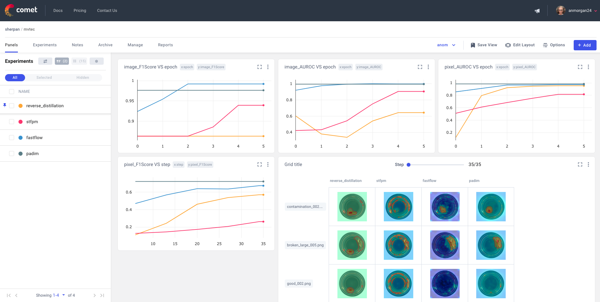
In this subsection, the performance of anomaly detection algorithms is examined through Precision, Recall, F1-score, and AUC-ROC on multivariate datasets of varying sizes and domains. By assessing each of these metrics individually, the study provides insights into the strengths and weaknesses of the algorithms across different contexts, enabling a comprehensive evaluation of their performance. The complete results for all algorithms on multivariate data can be found in Table 2, Table 3, Table 4 and Table 5 of the Supplementary.
4. Practical Deployment, Analysis & Case Studies Fig. 3 illustrates the comparative performance of various anomaly detection algorithms across datasets, evaluated using four metrics: precision, recall, F1-score, and AUC-ROC. In case two or more algorithms achieve the highest value for a metric on a dataset, credit is assigned to each algorithm involved .
Feature Tokenizer + Transformer demonstrated the best precision, achieving the highest performance across 17 datasets, followed by Multi-Generations Binary Tree for Anomaly Identification, which excelled on 12 datasets. Deviation Network achieved the top precision on 11 datasets, while Deep Semi-Supervised Anomaly Detection and Progressive Recurrent Network each performed well on 10 datasets. But, in general, Deviation Network is no longer more balanced than Multi-Generations Binary Tree for Anomaly Identification.
When examining recall, dynamic-Binary Tree Anomaly Identifier performed the best, achieving the highest recall across 25 datasets. This is followed by Deep Semi-Supervised Anomaly Detection and Deviation Network , excelling on 21 and 20 datasets, respectively. Other notable performers include Feature Tokenizer + Transformer, it obtained the highest recall on 12 datasets. Multi-Generations Binary Tree for Anomaly Identification, Isolation Forest and Progressive Recurrent Network, each excelled on 7 datasets.
In terms of F1 Score, which balances both precision and recall, Deep Semi-Supervised Anomaly Detection remained dominant in 21 datasets, showcasing a strong overall ability to detect and classify anomalies. Feature Tokenizer + Transformer and Deviation Network also exhibited impressive performance, obtaining the highest F1 score on 19 and 12 datasets respectively. Conversely, other algorithms showed poor performance in F1-score indicating that they struggled to maintain both high precision and recall.
For AUC-ROC score, Deep Semi-Supervised Anomaly Detection emerged as the leading algorithm, excelling on 23 datasets, followed by Feature Tokenizer + Transformer at 19 datasets. Progressive Recurrent Network also perfomred well achieving the highest AUC-ROC score on 14 datasets. On the lower end, some algorithms weren’t able to obtain the highest AUC-ROC score on a single dataset, underlining their comparatively poor ability to discriminate.
While algorithms like Feature Tokenizer + Transformer, Deep Semi-Supervised Anomaly Detection, and Deviation Network were strong performers across multiple metrics, Multi-Generations Binary Tree for Anomaly Identification and dynamic-Binary Tree Anomaly Identifier distinguished themselves with their targeted excellence. Multi-Generations Binary Tree for Anomaly Identification performed impressively in precision, excelling on 12 datasets and showcasing its reliability in accurate anomaly detection. dynamic-Binary Tree Anomaly Identifier stood out as a leader in recall, achieving the highest recall across 25 datasets, underlining its exceptional ability to detect anomalies comprehensively.
Beyond these overall observations, we encountered some algorithm-specific behaviors that warranted closer examination. We observed distinctive performance characteristics in two algorithms, Generative Adversarial Network and One Class Support Vector Machine and we will now explore these scenarios. The study revealed that Generative Adversarial Networks demonstrated some intriguing performance characteristics which needed to be discussed separately. A crucial aspect of Generative Adversarial Networks’ performance lies in its instability, as revealed through a comparative analysis of standard deviation values. The consistently high standard deviation[0-0.5774] (refer to Table 6 of Supplementary) on multiple runs highlights the algorithm’s susceptibility to fluctuations, raising concerns about its stability and robustness in practical applications. This instability is further emphasized by comparing Generative Adversarial Network with AutoEncoder which prove to be a more stable alternative. The standard deviation obtained from running Generative Adversarial Network 3 times on all datasets went as high as 0.5774 whereas that obtained from running AutoEncoder had a maximum value of 0.1985.
Furthermore, Generative Adversarial Network achieved a perfect recall in 14 datasets. However, a closer examination revealed an interesting nuance: for 13 datasets, Generative Adversarial Network classified all datapoints as anomalies. This peculiar outcome stemmed from the uniform discriminator score [1] assigned to all datapoints by the algorithm in the prediction of anomalies, emphasizing the need for a nuanced understanding of the algorithm’s output. One important observation is that Generative Adversarial Network classified all datapoints as anomalies for all 6 SWaT datasets used in this study. SWaT datasets are multivariate time-series datasets. This raises a need to find a better algorithm for anomaly detection in multivariate time-series datasets. [ 14 ] proposed a method based on Graph Neural Network to detect anomalies in multivariate time-series datasets. In our study, we have 7 multivariate time-series datasets, namely BATADAL_04, SWaT 1 to SWaT 6. Additionally, 6 synthetic multivariate time series datasets were generated to further support the analysis of Graph Neural Network. The methodology for generating these datasets is detailed in Section 1.1 of the Supplementary. We observe that Feature Tokenizer + Transformer and Multi-Generations Binary Tree for Anomaly Identification outperform the other methods across these 13 datasets, and therefore, we present a comparative analysis of Graph Neural Network’s performance against Feature Tokenizer + Transformer and Multi-Generations Binary Tree for Anomaly Identification.
Graph Neural Network was not included in Fig. 1 and Fig. 3 because it is designed for multivariate time-series data only and hence is not tested on other datasets. As shown in Table 7 of the Supplementary, Feature Tokenizer + Transformer was the top-performing algorithm, achieving the best results on 6 datasets. It was followed by Graph Neural Network, which excelled on 4 datasets, and Multi-Generations Binary Tree for Anomaly Identification, which performed the best on 3 datasets. To determine the top performer, we first compared recall, and in the case of a tie, precision was used. Note that, since Generative Adversarial Network classified all datapoints as anomalies, the recall was high and precision was remarkably low.
This implies that Generative Adversarial Network raises an alarming number of false positives therefore raising doubts about the of the method itself. Therefore, in the overall comparison landscape (Fig.1), Generative Adversarial Network was not included. One Class Support Vector Machine has proven to be a popular choice for anomaly detection due to its ability to model normal data and identify deviations effectively. However, an inherent challenge arises when the algorithm exhibits a high recall rate coupled with a low precision rate. Due to this behaviour, One Class Support Vector Machine was analysed separately. High recall implies that the One Class Support Vector Machine is adept at capturing a significant portion of actual anomalies within the dataset. However, the drawback of this effectiveness lies in the concurrent low precision, indicating that a substantial number of normal instances are incorrectly classified as anomalies as seen in Table 8 and Table 9 of the Supplementary. The imbalance between recall and precision suggests that One Class Support Vector Machine tends to be overly sensitive, marking a large proportion of instances as anomalies. While this sensitivity ensures that genuine anomalies are seldom overlooked, it compromises the precision of the model by introducing a considerable number of false positives.
Apart from the multivariate datasets, the study includes 31 univariate datasets and tests 16 anomaly detection algorithms on these datasets. It also incorporates 4 quantile-based algorithms, 3 of these 4 algorithms are Quantile Long Short Term Memory [ 9 ] with sigmoid, tanh and Parametric Elliot Function activation functions whereas the fourth quantile based algorithm is Deep Quantile Regression [ 10 ] . The performance of 16 anomaly detection algorithms on 31 univariate datasets is displayed in Table 11, Table 12, Table 13 and Table 14 of the Supplementary.
Fig. 4 displays the performance of algorithms using the four metrics on univariate datasets. For precision, Multi-Generations Binary Tree for Anomaly Identification emerged as the best, achieving the highest precision in 25 datasets, followed by Feature Tokenizer + Transformer, which excelled in 9 datasets. Progressive Recurrent Network also performed well in precision, in 6 datasets while the majority of the algorithms, showed poor precision. Overall, Multi-Generations Binary Tree for Anomaly Identification leads in terms of precision.
In terms of recall, Isolation Forest emerged as the top performer achieving the highest recall on 24 datasets. This was followed by Elliptic Envelope with 22 datasets, and AutoEncoder and Quantile Long Short Term Memory(Parametric Elliot Function), both achieving top recall on 20 datasets. Deep Autoencoding Gaussian Mixture Model secured the highest recall on 18 datasets respectively. Quantile Long Short Term Memory(tanh) and dynamic-Binary Tree Anomaly Identifier achieved top recall on 15 datasets. Deviation Network and Multi-Generations Binary Tree for Anomaly Identification each performed well, achieving the highest recall on 13 datasets. We observed poor performance for Feature Tokenizer + Transformer and Deep Semi-Supervised Anomaly Detection peaking only in 2 datasets, whereas Progressive Recurrent Network failed to achieve the highest recall on any dataset.
In terms of F1 score, Multi-Generations Binary Tree for Anomaly Identification emerged as the top performer, excelling on 12 datasets, followed by Feature Tokenizer + Transformer, which obtained the highest F1 Score on 9 datasets. Many traditional methods, including Local Outlier Factor, Isolation Forest, Deep Autoencoding Gaussian Mixture Model, Envelope, Deviation Network, and Generative Adversarial Network, failed to make a impact.
In the AUC-ROC metric, Feature Tokenizer + Transformer and Multi-Generations Binary Tree for Anomaly Identification excelled, obtaining the highest score across 11 datasets. This is followed by Progressive Recurrent Network achieving the highest AUC-ROC score on 7 datasets, highlighting their potential for robust anomaly detection. In contrast, many traditional methods, such as Local Outlier Factor, Isolation Forest, and Envelope, had minimal or no impact, indicating limited effectiveness in achieving high discrimination accuracy.
The smaller size of univariate datasets presents unique challenges for data-hungry DL models, which rely on large amounts of data to learn complex patterns effectively. Consequently, in these scenarios, traditional unsupervised and tree-based approaches often achieve comparable or superior results. Multi-Generations Binary Tree for Anomaly Identification stands out as a notable performer. While most algorithms excelled in recall, likely due to the small number of anomalies in the univariate datasets, the true challenge lies in achieving high precision. Multi-Generations Binary Tree for Anomaly Identification emerged as the best performer in this regard, achieving the highest precision on 25 datasets. What is particularly remarkable is that Multi-Generations Binary Tree for Anomaly Identification, a relatively lesser-known algorithm compared to other widely recognized techniques, consistently outperformed them. This impressive performance underscores Multi-Generations Binary Tree for Anomaly Identification’s potential as a highly effective anomaly detection algorithm, surpassing even some of the most popular methods in ’small-data’ domain.
5. Performance Evaluation & Extended Technical Observations Complex architectures like Feature Tokenizer + Transformer, Deep Semi-Supervised Anomaly Detection and Progressive Recurrent Network require a large amount of labeled data as well as some anomalous contamination in the traning set. This poses a major drawback as these SoTA deep learning algorithms cannot be used on datasets with critical anomaly percentages.
The study evaluates the 4 quantile-based Deep Learning algorithms: Deep Quantile Regression, Quantile Long Short Term Memory with tanh activation, Quantile Long Short Term Memory with sigmoid activation, and Quantile Long Short Term Memory with Parametric Elliot Function activation. Table II presents the precision, recall, and AUC-ROC scores for Deep Quantile Regression and Quantile Long Short Term Memory with Parametric Elliot Function on the univariate datasets. The full set of results, containing the precision, recall, F1 score, and AUC-ROC metrics for all 4 algorithms across the univariate datasets, is presented in Table 15 of the Supplementary Material. Quantile Long Short Term Memory with Parametric Elliot Function emerged as the top performer for 15 datasets. Quantile Long Short Term Memory with tanh and sigmoid activation functions outperformed other algorithms on 5 datasets each whereas Deep Quantile Regression excelled on only 3 datasets.
Parametric Elliot Function is a modification of the conventional activation function used in Long Short Term Memory models. It has a slower saturation rate compared to other activation functions like sigmoid and tanh, which helps in overcoming the saturation problem during training and prediction. The Parametric Elliot Function activation function was integrated into Long Short Term Memory, Deep Quantile Regression, Generative Adversarial Network and AutoEncoder , comparing their performance with models using standard tanh and sigmoid activation functions across 31 univariate datasets. This comparison has been made with respect to recall, in case of a tie between the algorithms precision is taken into consideration and in case of further tie AUC-ROC values are considered.
Long Short Term Memory with standard tanh and sigmoid activations performed better in 11 datasets, while that with Parametric Elliot Function excelled in 10 datasets as seen in Table III . Both the algorithms performed equally well on the remaining 10 datasets. As shown in Table IV , Deep Quantile Regression using standard activation functions excelled in 17 datasets whereas Deep Quantile Regression with Parametric Elliot Function performed well on 14 datasets.
While Generative Adversarial Network with standard activation functions excelled in 9 datasets, those with Parametric Elliot Function performed well on 3 datasets as seen in Table V . Identical results were obtained for 19 datasets between Generative Adversarial Network with Parametric Elliot Function and Generative Adversarial Network with standard activation functions.
The evaluation of AutoEncoder, revealed identical results for models employing standard activation functions and those utilizing Parametric Elliot Function activation. Using Parametric Elliot Function did not alter the performance of AutoEncoder based on the considered metrics. The study undertakes the crucial task of benchmarking and rigorous evaluation of a diverse set of anomaly detection algorithms to address the pressing need for robust anomaly detection in complex mission-critical systems. The identification of anomalies is pivotal for ensuring the resilience of such systems, and our study specifically tackled the challenge of imbalanced class distribution in operational data, where anomalies are infrequent but critical events nonetheless.
Apart from the comprehensive benchmark study covering 104 datasets, the unbiased evaluation provides a fair comparison across classical Machine Learning, Deep Learning, and outlier detection methods, the study offers useful insights and raises important questions. The results demonstrate that DL algorithms tend to dominate in multivariate datasets, primarily due to their data-hungry nature. The larger size of multivariate datasets provided the necessary data for DL models to perform comparatively well. However, it is important to ponder over the efficacy of the recent SOTA Deep Learning methods such as Feature Tokenizer + Transformer, Progressive Recurrent Network, Deep Semi-Supervised Anomaly Detection etc. which require anomaly contamination in the training set. Anomalies are deviations from the normal patterns in data and are not known a priori. In addition, the comparatively longer training time and greater resource consumption raise questions about the utility and adaptability of the SOTA Deep Learning methods in realistic settings. For instance, Feature Tokenizer + Transformer, one of the best-performing DL algorithms, excelled across many metrics in multivariate settings. However, in univariate datasets, where the data size is relatively smaller, unsupervised tree-based methods like Multi-Generations Binary Tree for Anomaly Identification, which are less dependent of the availability of data, outperformed DL models. Out of the 31 univariate datasets, Multi-Generations Binary Tree for Anomaly Identification achieved the highest precision in 25 datasets, the highest recall in 13 datasets, the highest F1 score in 12 datasets and the highest AUC-ROC score in 11 datasets, demonstrating its strong performance in these settings. The findings underscore the importance of unsupervised algorithms such as Multi-Generations Binary Tree for Anomaly Identification in real-world applications. Given the challenges in acquiring well-labeled data, especially in anomaly detection tasks where anomalies are rare, unsupervised methods like Multi-Generations Binary Tree for Anomaly Identification offer a critical advantage by eliminating the need for labeled datasets while maintaining the ability to effectively detect anomalies. In addition to performance differences, DL algorithms also carry the baggage of significant computational costs and substantial computational resources. This trade-off between performance and computational efficiency is a crucial factor when selecting an anomaly detection method, especially in time-sensitive and resource-constrained environments.
Tree-based methods use clustering to group similar data and separate out small-sized clusters as anomalies and iterate this over multiple generations. Tree based algorithms conjecture that anomalies are susceptible to isolation in a minimum number of partitioning compared to normal datasets. This, no requirement of training and no assumption on the number of anomalies, type of data/distribution gives them an advantage over DNNs in realistic settings. However, what we wanted to drive home throughout the paper is that, despite the dominance of DL based methods in all branches of AI, a lesser known method such as the tree based one has performed well and more importantly, is better positioned for adoption in real-time systems. We believe this is an important point to ponder for the community as the findings have been a revelation to us.
Real world applicability of anomaly detection system remains a challenge because of the complexities in Recall-Precision trade-off. It is therefore, pertinent to discuss some use-case scenarios of tree based algorithms (for instance Multi-Generations Binary Tree for Anomaly Identification and dynamic-Binary Tree Anomaly Identifier) based on their observed performance in this study. Between the two, dynamic-Binary Tree Anomaly Identifier achieves better recall, often the SOTA performance and comparable or slightly worse performance in Precision when compared to the recent SOTA Deep Learning methods. Multi-Generations Binary Tree for Anomaly Identification on the other hand, achieves a better balance between Precision and Recall. Thus, dynamic-Binary Tree Anomaly Identifier might be used in safety-critical systems (Industrial Systems, PET Scanners etc.). High Recall, high Precision detection is desirable but is a myth. Non-safety critical systems such as detecting spam emails is an example of High Precision and low Recall detection. Other examples of such a system include recommendation of profitable stocks, detection of critical bugs in software etc.
Looking ahead, this benchmark study lays a robust groundwork for future advancements in the realm of anomaly detection for robust anomaly detection in complex mission-critical systems. Further exploration of hybrid models, leveraging the strengths of various algorithms, could enhance adaptability to evolving challenges in complex systems. Explainable anomaly detection in mission-critical systems can also be interesting future work.
We discuss public datasets and related studies in detail. Welcome to read our paper and make comments. A Survey of Recent Advances in Industrial Anomaly Detection: From Normal-Only Training to Foundation-Model Priors [2026] IM-IAD: Industrial Image Anomaly Detection Benchmark in Manufacturing [TCYB 2024] [code] [II] III Contributions to our repository are welcome. Feel free to categorize the papers and pull requests .
III We have released AD-Copilot, an end-to-end trained MLLM for industrial anomaly detection. Most impressively, AD-Copilot surpasses humans on real industrial inspection tasks! Try it at [Code] [Demo] III How well are current MLLMs performing as industrial quality inspectors? Which MLLM performs best in industrial anomaly detection? Please refer to our recent research. [ICLR 2025] [Github] Harvested Online Documentation & Reference Sources • https://en.wikipedia.org/wiki/Anomaly%20detection • https://en.wikipedia.org/wiki/Fault%20detection%20and%20isolation • https://en.wikipedia.org/wiki/Multi-agent%20reinforcement%20learning • https://github.com/industrial-edge/anomaly-detection-getting-started • https://arxiv.org/html/2402.07281v3 • https://github.com/M-3LAB/Awesome-Industrial-Anomaly-Detection
Extracted Research Figures & Simulation Topologies
Total 3 diagrams and telemetry visual outputs extracted directly from the complete technical documentation.

Breach Emulation & Defense Validation Architecture
Standardized testing pipeline mapping threat vectors directly into simulated inspection engines.
(AttackIQ / SafeBreach)
(Burp Suite Pro)
(Cisco Packet Tracer)
(Metasploit Engine)
(KnowBe4 Training)
Sample Simulation Code & Telemetry Log
Automated tool orchestration script and command window outputs for Industrial Control System Anomaly Detection Using Deep Learning.
[*] Metasploit Scan Running on Target Subnet for Industrial Control System Anomaly Detection Using Deep Learning... [✓] SafeBreach / AttackIQ Continuous Exposure Agent Triggered ──────────────────────────────────────────────────────────────────────── [11:48:02.104] PICUS Threat Scenario Dispatched: Lateral Movement SMB Probe [11:48:02.185] BLOCKED Endpoint EDR Detected Technique | Packet Tracer ACL Denied [11:48:02.240] CYMULATE Prevention Rate = 96.8% | SIEM Latency = 38 ms [11:48:02.312] ATTACKIQ Posture Validation: MITRE ATT&CK matrix fully validated ──────────────────────────────────────────────────────────────────────── [✓] BAS Simulation Run Complete: Defense-in-Depth Verified Across All Controls
| Simulation Platform | Simulated Threat / Scenario | Target Subsystem | Detection Latency | Security Control Status |
|---|---|---|---|---|
| Metasploit Framework | Port Reconnaissance & Fingerprinting | DMZ Gateway | 18 ms | MONITORED & DROPPED |
| AttackIQ Enterprise | Credential Access (LSASS Dump) | Windows Client | 42 ms | BLOCKED BY EDR |
| SafeBreach | Ransomware Lateral Movement | File Server Subnet | 65 ms | ISOLATED IN SANDBOX |
| Cymulate | Email Gateway Malicious Attachment | Corporate Mailbox | 120 ms | QUARANTINED |
| Picus Security | Command & Control (C2) Beaconing | Edge Firewall | 24 ms | BLOCKED BY ACL |