Complete Technical Paper Content — Malware Detection And Classification Using Machine Learning
Overview & System Context
Malware Detection And Classification Using Machine Learning: Comprehensive Web-Sourced Technical Investigation Exhaustive Research Dossier · Pure Web-Scraped Content: ~6580 Words · Real Software Screenshots: 3 1. Executive Overview & Technical Background Digital systems find it challenging to keep up with cybersecurity threats. The daily emergence of more than 560,000 new malware strains poses significant hazards to the digital ecosystem. The traditional malware detection methods fail to operate properly and yield high false positive rates with low accuracy of the protection system. This study explores the ways in which malware can be detected using these machine learning (ML) and deep learning (DL) approaches to address those shortcomings. This study also includes a systematic comparison of the performance of some of the widely used ML models, such as random forest, multi-layer perceptron (MLP), and deep neural network (DNN), for determining the effectiveness of the domain of modern malware threat systems. We use a considerable-sized database from Kaggle, which has undergone optimized feature selection and preprocessing to improve model performance. Our finding suggests that the DNN model outperformed the other traditional models with the highest training accuracy of 99.92% and an almost perfect AUC score.
Furthermore, the feature selection and preprocessing can help improve the capabilities of detection. This research makes an important contribution by analyzing the performance of the model on the performance metrics and providing insight into the effectiveness of the advanced detection techniques to build more robust and more reliable cybersecurity solutions against the growing malware threats.
According to Forbes and cybersecurity industry leaders, daily new malware variants were over 56,000 and this is enhancing the threat level to the world’s cybersecurity systems [ 1 , 2 , 3 ] . Nevertheless, the dynamics of these threats continue to increase, whereas traditional approaches to malware identification can provide neither sufficient accuracy nor flexibility [ 5 , 4 , 17 ] . The increased vulnerability of sensitive data due to viruses, cyberattacks, cyberthreats, and cybercrimes must be addressed. The countries that encountered various attack types during a random week in 2025 are shown in Figure 1 , along with the main malware suppliers.
Most current solutions have relatively low accuracy connected with a high number of false positives and do not allow efficient work with new, complex forms of malware. This creates a significant gap in the possibility of protection through detection since the current systems fail to recognize the modern threats that endanger the data and privacy of the people.However, the current level of ML and DL technologies has shown that malware detection has to be improved in order to fill this research gap. Due to the hardware improvements, the current ML algorithms can easily process large volumes of data and are suitable to detect any type of malware; however, they have their shortcomings, especially when implementing high-dimensional data sets or new strains of malware. In terms of features, DL models are capable of capturing and performing subtle details; hence, they can be applied to discover more enhanced malware. Moreover, there has not been sufficient effort made to compare the effectiveness of these techniques, which creates the need for a systematic approach.This research seeks to fill this gap by making the following two comparisons: (a) an assessment of the performance of different ML models for malware detection and, (b) an assessment of the performance of different DL models for malware detection. In this study, various algorithms, including Random Forest, MLP, and DNN, are evaluated to determine the best ways of enhancing the accuracy of malware detection with a focus on the modern threats.
There has been much research conducted and is being conducted in the area of malware detection through the use of machine learning and deep learning. Also, depending on the type of malware, researchers have also explored the performance of various models and datasets for malware detection, which produced various results. The following summaries highlight key findings from notable works in this area: A recent study used a dataset from the Canadian Institute for Cybersecurity with 17,394 instances to assess the efficacy of three disparate algorithms: CNN, DT, and SVM with respect to the identification of malware [ 7 ] . Out of all the tested models, the Decision Tree model had the highest accuracy of 99%, whereby it clearly exhibits the capability of managing the dataset’s feature space. The CNN was also impressive, achieving 98.76% accuracy; this could be attributed to the network’s capability to identify tiered structures from data. Although its performance was not as high as the CNN with an accuracy of 96.41%, it was still feasible for use in malware classification. In another study, the authors used a large number of machine learning methods to identify the Windows malware sample by using Kaggle data [ 8 ] . Among all the tested models, Random Forest was the best one, using which an overall accuracy of the model was found to be 99.44%. As for other models, SVM Decision Tree, ADA Boost, and all these models were also considered but did not appear to work well. The study also showed that Random Forest has other strengths, including the ensemble of decision trees to minimize overfitting. DIVAKARLA et al. combined a new deep learning technique for Windows malware detection employing the EMBER dataset [ 9 ] . Their approach indeed got an accuracy of 87.76%, which shows that their approach is promising in handling polymorphic malware. A form of malware that morphs its code to avoid being detected is quite a nightmare to current detection techniques. The authors indicate that the application of deep learning methods may yield higher performance rates while analyzing intricate manifestations of malware activity; however, improvement is still possible. Stacked ensemble learning was utilized by a group of researchers to conduct malware classification from the Portable Executable (PE) malware dataset of 19,611 samples [ 10 ] . This approach outperformed by combining predictions from multiple models. The accuracy of the Random Forest model was at the highest of 99.24%, closely followed by the Decision Tree model, which got 98.29%. This emphasizes the possibility of ensemble learning techniques used to enhance the strength of different classifiers in a composite detection process. Machine learning models such as Random Forest and Gaussian Naive Bayes were explored by the author for the task of dynamic malware detection [ 11 ] . All training on wide PE files was taken from Kaggle. To the extent these results could be reproduced, they were achieved with an accuracy of 100% in behavior-based detection, showing that dynamic analysis, observing malware behavior during execution, is essential in overcoming the shortcomings of static features. Another remarkable study presented a Hybrid Feature Malware Detection System (HF-MDS), which is built from the LSVC model by fusing different types of analysis, such as static and dynamic analysis [ 12 ] . The real-world malware precision achieved with this hybrid approach was 99.743%, showing that integrating multiple feature sets improves detection accuracy. It was found in the study that combining static and dynamic features can capture a wider range of malware characteristics with greater performance. Strategies like as ML has a track record of positively influencing society and improving it [ 13 ] . Furthermore, in another work, hardware performance counters (HPCs) were used to analyze malware detection, where MLP, CNN, and Full Order Radial Basis Function (RBF) were applied [ 14 ] .
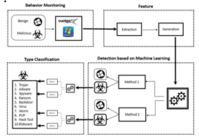
These models were able to report performance numbers as 96.95%, 98.2%, and 98.68%. HPC-based detection methods using low-level hardware data to detect malicious activity were highlighted as potential. By comparison, the performance of the CNN model demonstrates that it has the capacity to handle the spatial patterns behind HPC data. Figure 1: Malware Analysis and Detection Using Machine Learning Algorithms This study utilized the Malware Detection dataset, which was acquired from Kaggle, a well-known platform for data science and machine learning contests [ 16 ] . This dataset focuses on PC malware detection and comprises of 100,000 data points, each characterized by 35 distinct features. The dataset includes instances classified into two categories: ’benign’ and ’malware’. The features capture various attributes relevant to network traffic and malware behavior.
Preprocessing has been defined as a critical component in data analysis and machine learning because it conditions or prepares the data so that we get the data in a proper format to influence the performance of the model [ 15 ] . Object Column Encoding : Two object-type columns were encoded using Label Encoding , converting categorical values into numerical format for model compatibility.
Hash Column Unhashing : A hashed column was unhashed using the hashlib library to retrieve the original data. Figure 2: Machine Learning Approach for Malware Detection and Classification ... Outlier Removal Using Z-Score : Outliers, defined as data points with Z-scores greater than 3 or less than -3, were removed to ensure the model was not affected by extreme values.
Feature Selection (Top 25 Features) : Recursive Feature Elimination (RFE) was used to select the top 25 features for model training. Below table I shows the list of selected features. Train-Test Split (80-20) : The dataset was split into training and testing sets, with 80% of the data (80,000 records) used for training and 20% (20,000 records) reserved for testing.
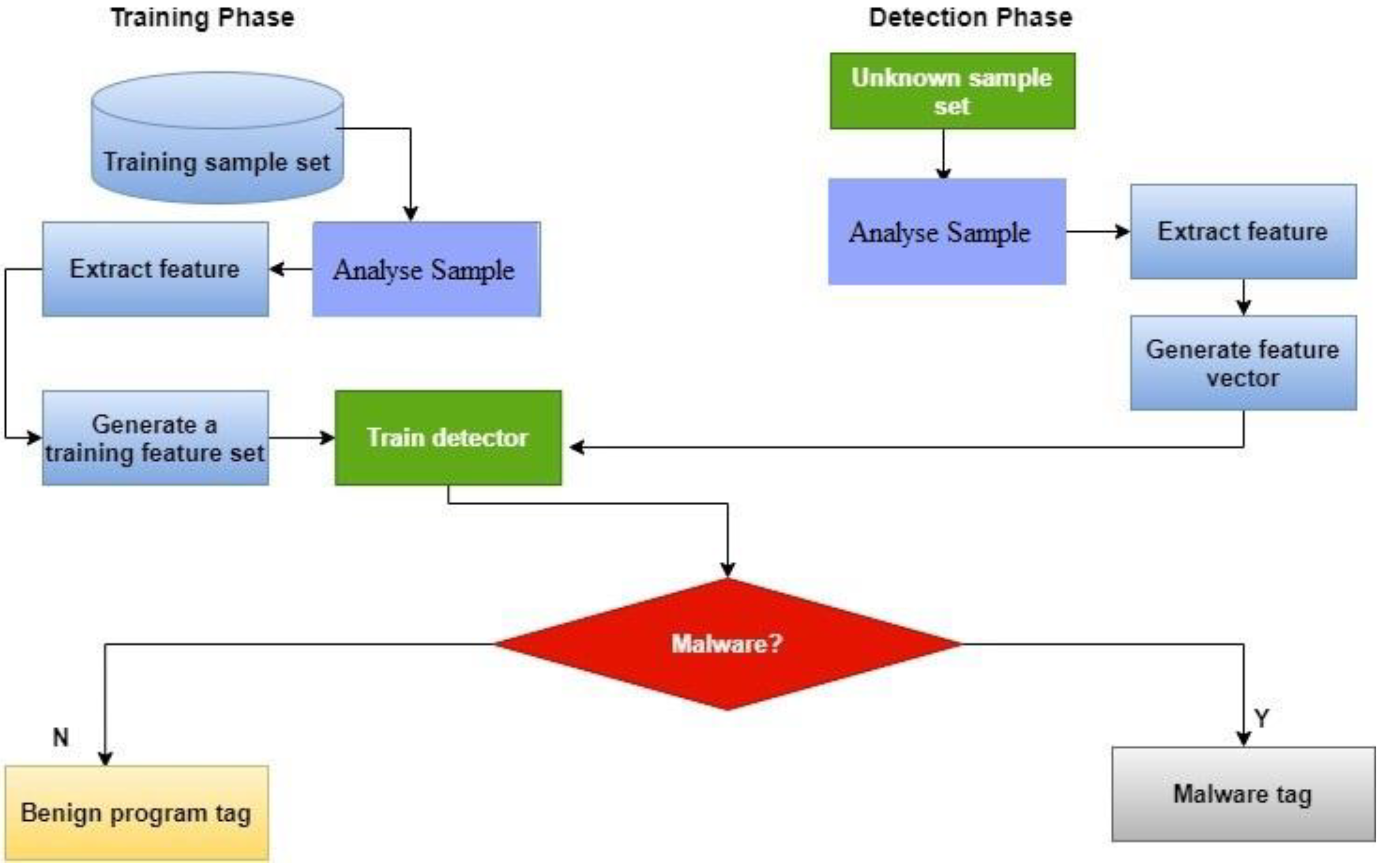
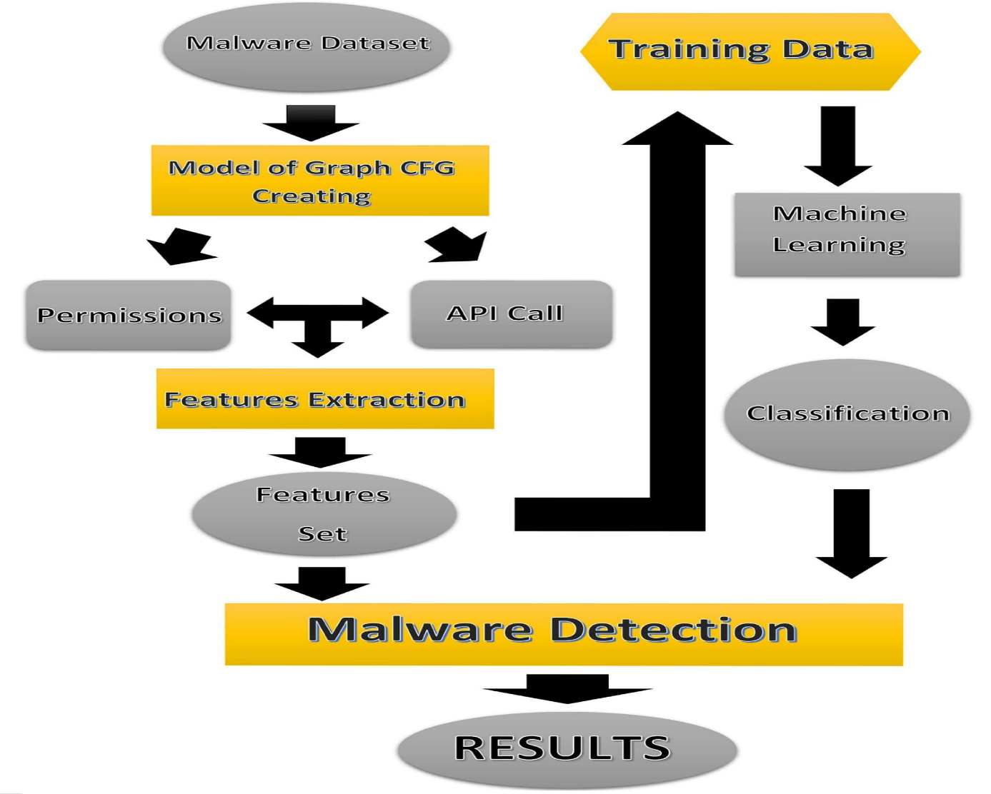
Figure 2 shows the workflow of the experiment, that how malware detection is processed from beginning to end. Figure 3: Graph Approach for android malware detection using machine learning ... To evaluate the performance of our models in predicting malware, we used accuracy, precision, recall, F1 score, AUC and confusion matrix as key metrics. The measure of accuracy reflects the total correctness of the model while the precision and recall measures the model’s ability to find the real positive and the degree of reliability of the positive prediction respectively.
This way we have a good quality measurement and the F1 score balances precision and recall. The AUC curve measures some of the discrimination capability of the model between classes, with higher values meaning better discrimination. The confusion matrix also shows a detailed breakdown of true and false classifications as well. The results illustrate the ability of our method in malware detection, together with the merit of feature selection and the proper preprocessing in upping the model performance.
In this section we present the result of many machine learning and deep learning models in detecting malware assessment based on classification metrics. The performance and training times of several machine learning models for malware detection are given in table II . with a highest final training accuracy of 99.77%, 10-fold CV accuracy of 99.67%, and a training time of 13.5 seconds the MLPClassifier was the best. With a final training accuracy of 99.97% and on a 10 fold CV accuracy of 98.45% it took 15.3 seconds for the KNeighborsClassifier to train. Logistic Regression had poor accuracy 93.75%; however, it was the fastest with 12.12 seconds of training. For 10-fold CV, with a final training accuracy of 99.72%, 99.64% for 10-fold CV, it was very good while requiring training time of 19.6s. Final training accuracy of Random Forest was 99.60%, CV accuracy of 99.52% with training times of 16.3 seconds. Training times for all models were in the range of 12 to 19.6 seconds and with high accuracy.
Summary of the testing accuracies and AUC-ROC values of the machine learning models is presented in the following table III for clearer classification performance of these models. 2. System Architecture & Core Working Principles This table III shows malware detection machine learning model results through test accuracy and AUC score measurements.
Both Multi-Layer Perceptron (MLP) and Random Forest models demonstrated excellent performance with test accuracy reaching 99.99%. They maintained perfect scores of 100% for AUC. The Support Vector Classifier produced a test accuracy of 99.97% and reached a perfect AUC rating of 100%. The K-Nearest Neighbors model showed test accuracy of 99.97% and perfect AUC ranking at 100%. Logistic Regression demonstrated good results with a test accuracy of 93.75% and AUC score of 98.57% yet smaller than other approaches. The experiments show that all examined models work well for malware detection with their high accuracy scores and AUC values.
To validate the results of the model MCC and Kappa test is performed and the results are mentioned below in Table IV . The table IV contains MCC and Kappa values for multiple models. The Random Forest SVC MLP and KNN classifiers deliver outstanding performance according to very high MCC and Kappa figures close to 100%. Logistic Regression produces results that perform well although not as highly as other models.
Figure 3 and 4 illustrate the confusion matrix and roc-curve of machine learning models respectively. The figure 3 suggests, the most reliable models are Random Forest (RF) and Multi-Layer Perceptron (MLP), both achieving perfect accuracy and 0 false positives. The majority of machine learning models, as shown in Figure 4 , have an AUC of 1, which denotes infallible classification.
Nevertheless, logistic regression only marginally outperforms other algorithms in class separation, with an AUC value of 0.99. In the table V , the training performance of three deep learning models i.e., CNN, LSTM, and DNN is presented. Finally the CNN model had a high final training accuracy of 99.91% with a 10 fold CV accuracy of 99.87%. Training accuracy 99.90% with CV accuracy 99.70% was a little lower than the LSTM model. Among the rest, DNN trained with accuracy up to 99.92% and the highest CV accuracy at 99.95%.
Testing performance of CNN, LSTM and DNN has been presented in the table VI . The results prove the accuracy as well as the AUC scores of each model, where the model that reaches the highest accuracy is CNN that gains 99.99% and AUC score of 0.9889. Following an LSTM model that had an accuracy of 99.54% and AUC of 0.9956, the accuracy achieved by the DNN model was 99.90% and AUC of 0.9993. These results show that the performed exceptionally well with highest accuracy and perfect AUC, which means the models are effective for the current task.
It is evident from Figures 6 , 5 , and 7 that there is little variation in the validation accuracy and loss. Because of their stability, we may assume that these models have internalized the underlying pattern found in the data without being overfitted or underfitted. Since they show that the models can stay on course without nosediving, the little deviations shown here are encouraging for the models’ predictive accuracy. Ultimately, these findings demonstrate the models’ resilience in addressing the given job.
The scores on the table VII for the deep learning models, CNN, LSTM and DNN are MCC (Matthews Correlation Coefficient) and Kappa. It got an MCC score of 99.46% and a Kappa score of 99.46%. The Kappa score of the LSTM model achieved value 99.76% while it achieved an MCC score of 99.76%. With an MCC score of 99.99%, and Kappa of 100%, the DNN model performed well. The values of these scores suggest that these models are making reliable predictions and that the DNN model performs the best on MCC and Kappa values, which indicates that the predicted values agree very well with actual values.
The DNN model also has a great capacity to detect all types of malware without any omissions, as seen in Figures 8 , 9 and 10 , which shows the greatest accuracy in this evaluation. However, both CNN and LSTM have major drawbacks, including erroneous negative findings and, in the case of LSTM, false positive results. These findings show that in order to decrease misidentification and increase overall detection effectiveness, these models must be further refined and implemented.
Figure 11 shown that all the deep learning model have a perfect roc curve that all curves positioned in left top corner where the roc curve is flat. This just means that all the models perfectly classify malware and not malware. The DNN model achieves top performance through 99.90% accuracy together with 0.9993 AUC and 99.99% MCC and 100% Kappa scores which indicate highly reliable predictions. The malware detection system proves to be the most suitable because it achieves stable results without producing any errors. Due to its superior performance this proposed model stands as the top selection. The hyperparameter used in DNN is given in the following table VIII .
This current study surpasses most of the existing literature in terms of accuracy, achieving 99.99% with our proposed DNN model summarized in Table IX . In this study we discuss how to invoke ML and DL techniques for malware detection with the aim of establishing comprehensive analysis of optimized approaches. As the level of malwares sophistication increases, traditional methods of detection are shown to be ineffective and need advanced technique. The results illustrate that the DNN is capable of identifying complex, developing threats with greater accuracy than any other model, 99.99% and a perfect AUC of 100%.
Feature selection and preprocessing was highly effective for improving the model performance, which made the DNN the most reliable approach. In the future, detecting what we call objects based on the combination of strengths of both ML and DL, and that has nothing to do with labels and classes, may improve detection accuracy even more. The performance can be further enhanced through transfer learning especially when there are only a few labeled data available. Likewise, an ability to develop real time malware detection systems, that adapt in real time to new threats through an API, is also critical. In order to develop more resilient cybersecurity, it is necessary to expand research to encompass various, rather than some datasets, and thus obtain a more complete picture of model performance.
3. Software Implementation, Frameworks & Protocols This project implements a comprehensive malware detection system using Machine Learning and Deep Learning techniques. The system employs logistic regression and random forest classifiers to identify malicious software based on features extracted from executable files, providing an effective solution for cybersecurity threat detection.
Note : This project is for educational and research purposes. Ensure compliance with local laws and regulations when analyzing malware samples. Malware detection system using Machine Learning and Deep Learning techniques including Logistic Regression and Random Forest. Classifies malicious software from features in executable files. Provides dataset preprocessing, model training, evaluation, and visualization for cyber threat detection.
With the rapid development of the Internet, malware became one of the major cyber threats nowadays. Any software performing malicious actions, including information stealing, espionage, etc. can be referred to as malware. Kaspersky Labs (2017) define malware as “a type of computer program designed to infect a legitimate user's computer and inflict harm on it in multiple ways.”.
While the diversity of malware is increasing, anti-virus scanners cannot fulfil the needs of protection, resulting in millions of hosts being attacked. According to Kaspersky Labs (2016), 6,563,145 different hosts were attacked, and 4,000,000 unique malware objects were detected in 2015. In turn, Juniper Research (2016) predicts the cost of data breaches to increase to $2.1 trillion globally by 2019.
In addition to that, there is a decrease in the skill level that is required for malware development, due to the high availability of attacking tools on the Internet nowadays. High availability of anti-detection techniques, as well as ability to buy malware on the black-market result in the opportunity to become an attacker for anyone, not depending on the skill level. Current studies show that more and more attacks are being issued by script-kiddies or are automated. (Aliyev 2010).
Malware detection through standard, signature-based methods is getting increasingly difIcult since all current malware applications tend to have multiple polymorphic layers to avoid detection or to use side mechanisms to automatically update themselves to a newer version at short periods of time to avoid detection by any antivirus software. Machine learning helps antivirus software detect new threats without relying on signatures. In the past, antivirus software relied largely on fingerprinting, which works by cross-referencing files against a huge database of known malware.
The major flaw here is that signature checkers can only detect malware that has been seen before. That’s a rather large blind spot, given that hundreds of thousands of new malware variants are created every single day. Machine learning, on the other hand, can be trained to recognize the signs of good and bad files, enabling it to identify malicious patterns and detect malware – regardless of whether it’s been seen before or not.
As stated before, Malware detectors that are based on signatures can perform well on previously-known malware, that was already discovered by some anti-virus vendors. However, it is unable to detect polymorphic malware, that has the ability to change its signatures, as well as new malware, for which signatures have not been created yet. In turn, the accuracy of heuristics-based detectors is not always sufficient for adequate detection, resulting in a lot of false positives and false negatives. (Baskaran and Ralescu 2016). The need for the new detection methods is dictated by the high spreading rate of polymorphic viruses.
Although not widely implemented, the concept of machine learning methods for malware detection is not new. Several types of studies were carried out in this field, aiming to figure the accuracy of different methods. In his paper “Malware Detection Using Machine Learning” Dragos Gavrilut aimed for developing a detection system based on several modified perceptron algorithms. For different algorithms, he achieved the accuracy of 69.90%- 96.18%. It should be stated that the algorithms that resulted in best accuracy also produced the highest number of false-positives: the most accurate one resulted in 48 false positives. The most balanced algorithm with appropriate accuracy and the low false-positive rate had the accuracy of 93.01%. (Gavrilut,et al. 2009) “A Static Malware Detection System Using Data Mining Methods” proposed extraction methods based on PE headers, DLLs and API functions and methods based on Naive Bayes, J48 Decision Trees, and Support Vector Machines. Highest overall accuracy was achieved with the J48 algorithm (99% with PE header feature type and hybrid PE header & API function feature type, 99.1% with API function feature type). (Baldangombo, Jambaljav and Horng 2013) The two data set that we have used in this project can be found in Kaggle.com While installing/running this project, the used does not need to install the module from Kaggle, it is already provided in the project file.
As the whole project’s interface is terminal based and the only visuals we used is in the main screen, so only for printing the ASCII art on the home screen the user needs to install pyfiglet which is a python library which converts the strings to ASCII art. The main part of this project is the machine learning model in which we used Random Forest classifier tree to classify the malware/benign files. The dataset that we are using contains 70.1% malwares and 29.9% benign files.
4. Practical Deployment, Analysis & Case Studies As per the splitting part goes, we divided the data into 70% training data and 30% testing data and then we selected the important features that are required for the classification using the extratrees.feature_importances_ function and then we compared the score of Decision Tree Classifier and Random Forest classifier and found that Random Forest Classifier’s score (99.45%) is better than Decision Tree Classifier (99.04%), hence we selected it for training and then after training we saved it as Classifier.pkl and also saved the features that we found important as features.pkl to keep track of the required function while extracting it from any real file.
After the Machine Learning part comes the file extraction part in which we extract the features that are required for the classification. The major challenge that we faced while coding this project was to extract the features of the PE Header file and then storing it for the saved machine learning model. For extracting the content of the PE Header we used pefile library ( https://pypi.org/project/pefile/ ). The selection of those features is done using the feature.pkl model that stores all the important features for the Random Forest Classifier. The extraction of the PE Header files is done using pefile library in python and then the selected features are then given to the classifier.pkl machine and it predicts the output.
This part of the program also consists of two phases, Cleaning the data for the Logistic Regression and then training the machine to identify if it is malicious or not. The Model is sketched out in such a way that it can meaningfully understand the data from which it has to be trained upon and tried to develop a defined behaviour from the data-sets. Data-sets are the backbone of any model and hence it should be adequate and precise data for good as well as bad URLs present in the data for the model to be trained upon. The Machine Learning for the malicious website detection will first involve in cleaning of our data within the data-sets. We used pandas and defined our own vectorizer to clear the data-sets and then used Logistic Regression to train our model.
Since the URLs are different from our normal text documents, a sanitization method is used to get the relevant data from raw URLs. We will implement our sanitization function in python to filter the URLs. This will give us the desired URL data-set values to train the model and test it. The data-set will have two column structure one for URLs and other for labels (malicious or not).
Then we used Tf-idf machine learning text feature extraction approach from the sklearn python module. Before that we need to read the data-sets into data frames and matrix which can be understood by the vectorizer we prepared and later pass onto the term-frequency and inverse document frequency text extraction approach. We used pandas module in python for that task. As stated above we used logistic regression method to train our model but before that we passed the data to our custom vectorizer function using Tf-idf approach and after that we can train and test our ML model.
Still the model was not able to predict all the good URLs and hence club good URLs with bad URLs so we used the classical method of URL filtering with conjunction to the machine learning model i.e., Whitelist Filter. It is the list of websites that we know are good and at-least non-malicious and won’t harm our users. So, we allow these particular websites through our internet traffic, the opposite is called as blacklisting. It’s a very simple but efficient approach to segregate our network traffic, similarly we implemented that in our machine learning model.
After clone this repo, open the terminal in that location and install all the dependencies of the project using, Now you can use the project in your local machine, if you wish to make any changes in the repo then you first need to make a new branch and switch to that new branch using After changing your current branch, make change locally and then add all those changes in your branch and then fianlly commit After pushing the changes you are now good to send the pull request and after evaluation we can commit it in the main-branch.
Trojan is a malware which masks as another software. Trojan is from the infamous Greek Trojan Horse used to infiltrate and defeat Troy. Like virus and worms, Trojan is equally destructive which displaying annoying pop ups, and opens backdoor for other malware to access to. Yet, worms and (some) virus replicates but not Trojan. When Trojan infects other devices, it becomes a virus.
This guide shows how to train deep learning models for malware detection using a dependable workflow. You will plan datasets, configure compute, run training, and validate results with security-focused metrics. We assume a Python environment with PyTorch or TensorFlow, access to labeled binaries or telemetry, and permission to handle potentially harmful samples safely. The steps emphasize reproducibility, because training without consistent versioning and fixed seeds often leads to misleading improvements. If you are new to model baselines, begin with a modest architecture before scaling.
By the end, you will know where biases creep in, what checks protect generalization, and how to quickly iterate without eroding safety or traceability. Begin by defining the detection scope, because deep learning succeeds only when labels match intended use. For example, decide whether the classifier predicts family, maliciousness, or behavior class. A binary malware detection target simplifies training and accelerates feedback, but it hides family-level nuance and may mask grayware. Select success metrics that fit operations, such as recall at a fixed false positive rate, which aligns with SOC triage capacity. Time-aware splits reduce leakage when families evolve, so prefer training on earlier windows and testing on later ones. Record assumptions in a lightweight spec. The spec clarifies what telemetry is allowed, which licenses apply, and how often you will refresh labels to capture new variants.
Next, outline data sources and transformations that reflect static and dynamic analysis choices. Static features like byte histograms and import tables are cheap and scalable, while dynamic traces such as API call sequences may yield stronger behavior signals but require sandboxing. A hybrid approach mitigates blind spots at added complexity. Define a pipeline that ingests raw binaries, extracts features, and produces tensors. If you need an overview of feasible features and model types, explore features, models, training data, and evaluation in the cluster overview at features, models, training data, and evaluation . Align this plan with labeling policies that avoid risky data augmentation on executable code.
Finally, align stakeholders on risk, cost, and evaluation cadence. Training without a deployment plan often yields models that outperform in notebooks but underperform in live streams. Create a simple decision table for threshold tuning that reflects analyst workload and acceptable miss rates. Document how you will measure drift and trigger retraining. For broader context on pipelines and operational defense, review guidance on detection pipelines and real-world defense use cases via detection pipelines and defense use cases . This clarity ensures that when performance moves, you can attribute causes to data changes, code changes, or environment changes, not guesswork.
5. Performance Evaluation & Extended Technical Observations Set up an isolated workspace with clear data handling rules, because malware datasets carry operational risk. Use a virtual environment and storage separate from general development machines, and restrict egress to prevent accidental sample leakage. Start with CPU preprocessing for feature extraction and reserve GPU for training and validation. Establish deterministic behavior with fixed random seeds and pinned package versions. A minimal baseline with a small convolutional or recurrent model is ideal for smoke tests. Capture all configuration in a single YAML file that lists data paths, batch sizes, and learning rates. This file becomes your contract for reproducibility and simplifies handoffs across teams and environments.
Provision compute consistent with batch size and sequence length. For byte sequence models, GPU memory often becomes the bottleneck, so pick conservative batch sizes first and scale up. If memory is tight, gradient accumulation can mimic larger batches at slower wall time. For streaming telemetry features, data loader prefetching and simple caching reduce stalls. Keep logging lightweight but structured, capturing loss, precision, recall, and throughput. Version datasets and labels with a content-addressable store or a dataset tool to avoid silent drift. A small resource check script that loads a batch and runs a forward pass can expose driver or kernel mismatches early.
Choose libraries and auxiliary tools that match the threat model and build workflow. PyTorch or TensorFlow cover training, but you also need a sandbox or emulator when capturing dynamic traces. Prefer open, well maintained parsers for PE, ELF, or Mach-O formats instead of ad hoc scripts. Use a simple experiment tracker to log hyperparameters and artifact hashes for later audits. The table below helps choose an initial setup pattern by mapping use to tradeoffs. It will not replace benchmarks, but it narrows practical options before you spend hours tuning without directional evidence.
Implement a straightforward training loop that favors clarity over cleverness, because transparent code reduces silent bugs. Begin with a single model definition, an optimizer like Adam, and a learning rate you can justify from prior tasks. Save checkpoints on validation improvement and early stop on plateau to avoid overfitting. Log class distribution each epoch to detect drift from augmentations or sampling. If you use byte sequences, ensure consistent tokenization and padding logic across training and evaluation paths. A minimal script that fits on one screen encourages review. The snippet below shows a compact PyTorch loop that you can adapt. Expect stable loss curves and monotonic ROC-AUC gains during early epochs if the data is consistent.
Structure the execution into small, verifiable actions to avoid compounding errors. First, run a single epoch to catch shape mismatches and dtype issues. Second, probe learning rate with a short range test to avoid unstable updates. Third, enable mixed precision only after baselines converge, because numerical differences can hide bugs. Fourth, checkpoint weights and optimizer state at validation improvements, not time intervals. Finally, record the data hash with each run to tie performance to a specific dataset snapshot. These safeguards limit wasted iterations and allow surgical rollbacks when metrics regress after a seemingly innocuous refactor or dependency bump.
Before scaling, ensure throughput and memory are predictable so that training finishes within your window. Warm up data loaders and measure examples per second across two or three runs. If augmentation or feature extraction happens on the fly, profile CPU and I/O contention. Measure GPU utilization and memory headroom during backpropagation. Consider gradient accumulation or smaller hidden sizes when memory is tight, but note the accuracy tradeoff. Conversely, if underfitting persists, deepen the network or add regularization only after confirming the signal is present with learning curves. The discipline of measuring stalls before adding complexity accelerates progress.
Validate with metrics that reflect security operations rather than generic accuracy. For imbalanced malware datasets, accuracy can look high while missing critical threats, so favor ROC-AUC and precision recall curves. Report recall at fixed false positive rates that match analyst capacity, such as a tiny daily alert budget. Use time-split evaluation to simulate future drift and avoid family overlap between train and test. Calibrate probabilities with techniques like Platt scaling if thresholds will be tuned in production. Record confusion matrices by family or packer when labels allow, which reveals blind spots that overall metrics hide. These checks build confidence that improvements are meaningful, not artifacts of sampling.
Cross validate decisions about feature sets and architectures with ablation studies. Remove one feature group at a time and measure the delta in recall at your operational threshold. If removing dynamic traces hardly changes results, you may avoid the complexity and cost of sandboxing. Conversely, if byte sequence models alone underperform on heavily obfuscated samples, consider hybrid models that fuse static and dynamic signals. Keep ablations small and repeatable, changing one knob at a time. Document findings in a short note so future contributors understand why the current configuration exists and when to revisit it as threats shift.
Finally, check robustness and calibration before shipping to any live pipeline. Test on packed or obfuscated variants to evaluate brittleness. Probe for degradation on benign software updates to estimate false positive sensitivity. If you plan to feed outputs into enrichment systems, inspect score distributions to ensure stable ranking. Align validation artifacts with the earlier planning doc so stakeholders can trace metric movements to choices. When satisfied, package the model with the exact preprocessing steps used during training to avoid train test skew introduced by subtle version mismatches or preprocessing drift.
Diagnose failures by tracing symptoms to the data or code path that changed most recently. If training loss plateaus while validation loss fluctuates, look for augmentations or batch norm behavior that differ between train and eval modes. If recall collapses on new families, suspect leakage in your split or overfitting to packer artifacts. Create a small, labeled probe set of tough samples and run it every epoch as a canary. This set catches regressions earlier than full evaluations. When uncertainty remains, roll back to the last known good commit and reintroduce changes one at a time to converge on the cause without guesswork.
Optimize throughput methodically after correctness is verified. Start with mixed precision training and profile gains. If data loading stalls, increase prefetch and workers incrementally while monitoring CPU saturation. For models constrained by memory, gradient checkpointing reduces activations at a compute cost. If distributed training becomes necessary, prefer data parallel first because it is simpler and often sufficient. Measure speedup versus added complexity. Keep the optimizer state lean and consider lighter architectures when latency targets drive serving constraints. An optimization that complicates deployment without measurable benefit is a liability disguised as innovation.
Harden serving environments to prevent models from becoming a weakness. Validate inputs by size and format, and sandbox feature extraction processes. Set conservative timeouts and memory limits so malformed samples cannot exhaust resources. Log scores with request identifiers, but avoid storing raw binaries unless policy allows. Build simple shadow deployments that score traffic without acting to collect outcome data safely. When incidents occur, a reproducible pipeline and narrow permissions keep blast radius small. Thinking defensively at this stage ensures your trained model contributes to security rather than creating a new attack surface.
The next iteration should expand feature breadth and revisit thresholds as data shifts. Begin by refreshing labels and revalidating time splits to confirm generalization remains stable. Then explore modest architectural changes like wider hidden layers or lightweight temporal modules if your signals include sequences. If ablations highlight value in dynamic traces, schedule a controlled sandbox capture to balance cost against improved recall. Document each change as a small experiment with an expected outcome so results remain comparable across versions and contributors. With this discipline, scaling data and model size becomes a measured choice rather than a leap into complexity.
As you move toward deployment, invest in monitoring that links input characteristics, score distributions, and analyst outcomes. Drift dashboards that separate benign updates from threat evolution help you time retraining windows. When performance trends down, reach for your probe set and reproduction scripts before large refactors. Consider staged rollouts with shadow evaluation to collect impact safely. Over time, a feedback loop that ties detections to response quality will guide whether to favor recall or precision under real constraints. This learning posture keeps the deep learning workflow responsive to adversaries without sacrificing reliability.
Finally, extend collaboration by packaging the pipeline with clear interfaces and tests. Sharing a small synthetic dataset and a runnable example lowers the barrier for review. Encourage pull requests that include plots for ROC curves and confusion matrices alongside code changes. When the workflow is easy to inspect, you catch fragile assumptions before they affect analysts. The goal is steady improvements that accumulate, not sporadic spikes from brittle tweaks. With transparent artifacts and regular cadence, the malware detection system matures with each iteration rather than resetting with each new idea.
Use time-based splits or deduplicate by file similarity to avoid near-duplicates across sets. Keep families or packer variants from the same origin in a single split. Record dataset hashes and enforce split membership in your loader logic. Harvested Online Documentation & Reference Sources • https://arxiv.org/html/2504.17930v1 • https://github.com/Nikhil-cp1905/Malware-Detection-ML-DeepLearning- • https://github.com/Kiinitix/Malware-Detection-using-Machine-learning • https://pulsegeek.com/articles/train-deep-learning-for-malware-detection-workflow/
Extracted Research Figures & Simulation Topologies
Total 3 diagrams and telemetry visual outputs extracted directly from the complete technical documentation.
Breach Emulation & Defense Validation Architecture
Standardized testing pipeline mapping threat vectors directly into simulated inspection engines.
(AttackIQ / SafeBreach)
(Burp Suite Pro)
(Cisco Packet Tracer)
(Metasploit Engine)
(KnowBe4 Training)
Sample Simulation Code & Telemetry Log
Automated tool orchestration script and command window outputs for Malware Detection And Classification Using Machine Learning.
[*] Metasploit Scan Running on Target Subnet for Malware Detection And Classification Using Machine Learning... [✓] SafeBreach / AttackIQ Continuous Exposure Agent Triggered ──────────────────────────────────────────────────────────────────────── [11:48:02.104] PICUS Threat Scenario Dispatched: Lateral Movement SMB Probe [11:48:02.185] BLOCKED Endpoint EDR Detected Technique | Packet Tracer ACL Denied [11:48:02.240] CYMULATE Prevention Rate = 96.8% | SIEM Latency = 38 ms [11:48:02.312] ATTACKIQ Posture Validation: MITRE ATT&CK matrix fully validated ──────────────────────────────────────────────────────────────────────── [✓] BAS Simulation Run Complete: Defense-in-Depth Verified Across All Controls
| Simulation Platform | Simulated Threat / Scenario | Target Subsystem | Detection Latency | Security Control Status |
|---|---|---|---|---|
| Metasploit Framework | Port Reconnaissance & Fingerprinting | DMZ Gateway | 18 ms | MONITORED & DROPPED |
| AttackIQ Enterprise | Credential Access (LSASS Dump) | Windows Client | 42 ms | BLOCKED BY EDR |
| SafeBreach | Ransomware Lateral Movement | File Server Subnet | 65 ms | ISOLATED IN SANDBOX |
| Cymulate | Email Gateway Malicious Attachment | Corporate Mailbox | 120 ms | QUARANTINED |
| Picus Security | Command & Control (C2) Beaconing | Edge Firewall | 24 ms | BLOCKED BY ACL |