Complete Technical Paper Content — Network Anomaly Detection Using Isolation Forest Algorithm
Overview & System Context
Network Anomaly Detection Using Isolation Forest Algorithm: Comprehensive Web-Sourced Technical Investigation Exhaustive Research Dossier · Pure Web-Scraped Content: ~6712 Words · Real Software Screenshots: 3 1. Executive Overview & Technical Background As cyber threats continue to evolve in sophistication and scale, the ability to detect anomalous network behavior has become critical for maintaining robust cybersecurity defenses. Modern cybersecurity systems face the overwhelming challenge of analyzing billions of daily network interactions to identify potential threats, making efficient and accurate anomaly detection algorithms crucial for network defense. This paper investigates the use of variations of the Isolation Forest (iForest) machine learning algorithm for detecting anomalies in internet scan data. In particular, it presents the Set-Partitioned Isolation Forest (siForest), a novel extension of the iForest method designed to detect anomalies in set-structured data. By treating instances such as sets of multiple network scans with the same IP address as cohesive units, siForest effectively addresses some challenges of analyzing complex, multidimensional datasets. Extensive experiments on synthetic datasets simulating diverse anomaly scenarios in network traffic demonstrate that siForest has the potential to outperform traditional approaches on some types of internet scan data.
Protecting networks against cyber-attacks requires the correct identification of any potential weaknesses that could be exploited by attackers. Such vulnerabilities, collectively known as attack surface , may include open ports, exposed services, misconfigured systems, and third-party integrations. The growing use of interconnected systems and digital technologies, using AI-driven attacks, and applying zero-day exploits leads to a larger attack surface and makes its identification harder.
Hence, the use of automated systems capable of continuously monitoring, assessing, and mitigating vulnerabilities in real-time becomes essential. One way to identify attack surface vulnerabilities is by using machine learning (ML) techniques. ML can detect anomalies in the network traffic data, which may point to potential issues that need to be addressed. However, finding such anomalies is challenging due to the high-dimensional and variable nature of network data. Network scans often include multiple features per IP address, with significant variation in both quantity and type.
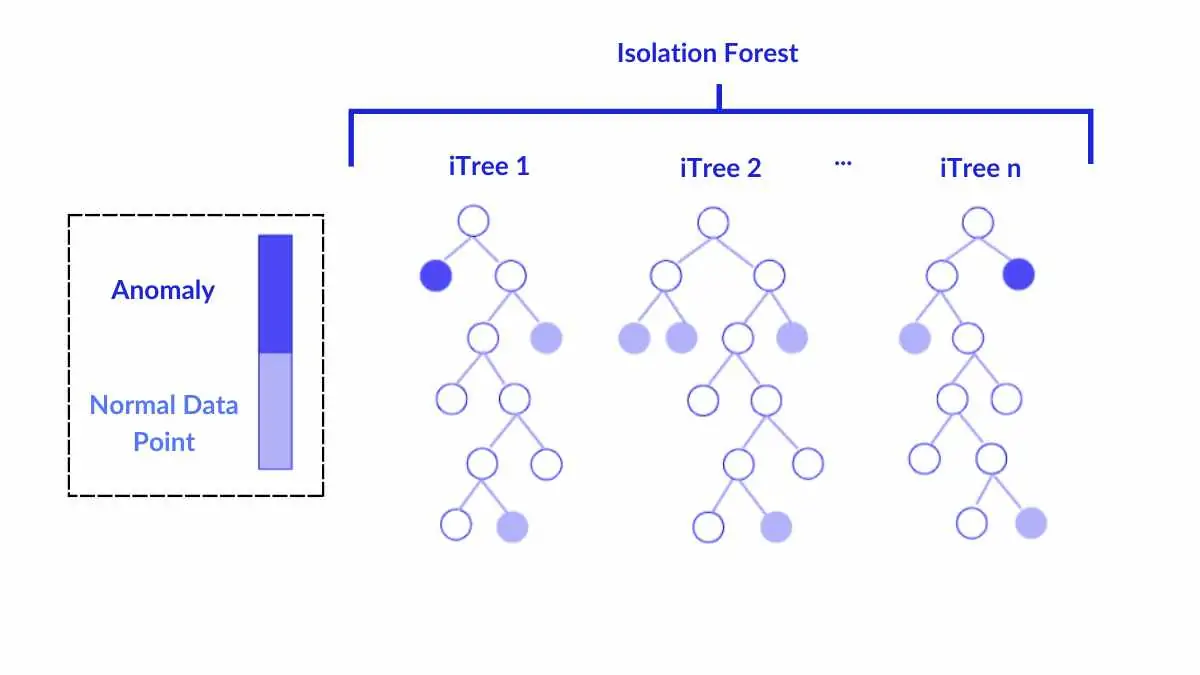
Machine learning techniques, such as clustering-based methods (e.g., k-means [ 17 ] , DBSCAN [ 12 ] ) and tree-based algorithms (e.g., Isolation Forest [ 20 ] , Random Forest [ 16 ] anomaly detection), are widely used to identify patterns that deviate from expected behavior. Figure 1: Isolation Forest Made Easy & How To Tutorial Isolation Forest (iForest) , which is one of the most scalable algorithms in this class, isolates anomalies by recursively splitting the data, and using the number of splits required to isolate a point as a measure of its anomaly score (Figure 1 ). Specifically, it constructs an ensemble of binary trees (a forest ) by randomly selecting a feature and a split value within the feature’s range at each node. The process continues recursively until a single point is left (the point is isolated) or a maximum tree depth is reached. Points closer to the root of a tree (requiring fewer splits for isolation) are considered more anomalous, while those deeper in the tree (requiring more splits) are likely part of dense clusters.
However, this method shows limitations when applied to more complex types of data such as network scan data. iForest assumes fixed-length feature vectors and numerical inputs, which makes it less effective for set-structured data where features like ports and services vary across IPs. To address these challenges, this paper introduces siForest, a variation of iForest designed specifically for set-structured data. The proposed method preserves the structure of the original data, and specifically the contextual relationships between ports and services under each IP. We experimentally compare siForest with two other implementations based on the original iForest implementation. The paper concluded with a discussion of the results and a list of tasks for further improvements.
Network security analysts increasingly rely on anomaly detection to identify threats in complex environments. The theoretical foundations for modern detection methods [ 9 ] , particularly those focusing on pattern recognition in security contexts, have evolved to address challenges in dynamic, large-scale networks where traditional approaches often fail [ 2 ] . Statistical methodologies [ 22 ] have proven especially effective in environments processing terabytes of network traffic daily while maintaining high accuracy rates.
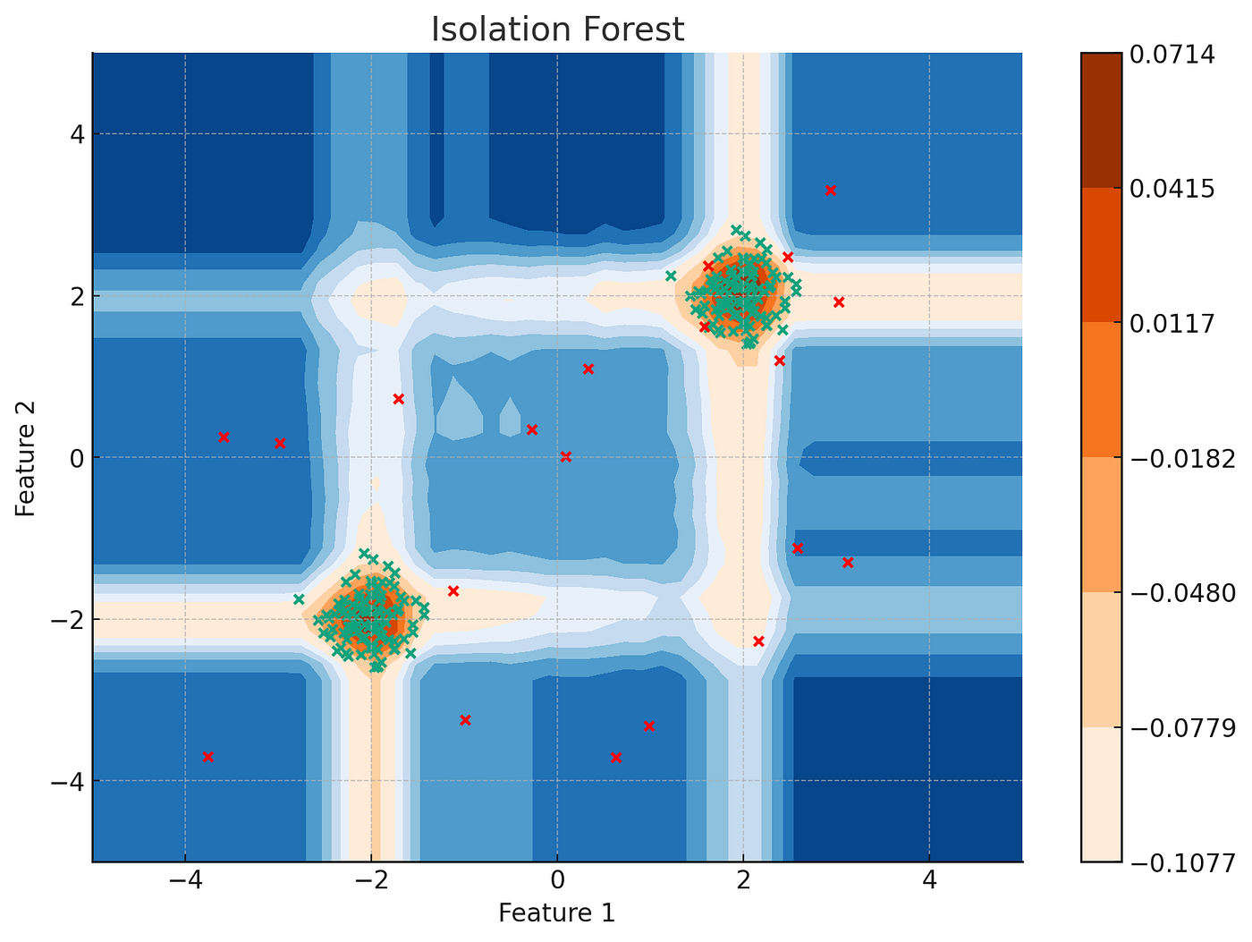
Figure 2: Isolation Forest The integration of machine learning has fundamentally changed anomaly detection capabilities, especially in analyzing high-dimensional data. While early research established core principles for identifying rare events [ 11 ] , recent advances in deep learning have revolutionized network traffic analysis through multi-layered pattern recognition [ 27 ] . Graph-based approaches [ 3 ] are particularly good at modeling complex relationships between objects of interest, using advanced node feature learning techniques [ 29 ] .
Within cybersecurity applications, these methods demonstrate better effectiveness against zero-day exploits and massive-scale traffic analysis. Research into generalization capabilities across different network behaviors [ 25 ] has revealed important insights for practical deployment. Deep hierarchical representations [ 5 ] prove especially effective at capturing subtle attack patterns, leading to broader applications across multiple security domains [ 19 ] .
Isolation Forest [ 20 ] is a more recent unsupervised machine learning algorithm particularly good at processing high-dimensional data. It’s main advantages are the high computational efficiency, while maintaining good accuracy. Further work [ 14 ] improved the algorithm’s resilience against complex attack patterns, and practical implementations [ 21 ] demonstrated its effectiveness in production environments. Recent benchmarking studies [ 31 ] analyzed the performance improvements across diverse scenarios.
Recent advances in graph-based detection have yielded promising results in network security applications. While earlier work explored basic graph structures for relationship modeling [ 3 ] , the development of graph convolutional networks [ 18 ] has dramatically improved detection accuracy in real-world security scenarios. These improvements, combined with advanced clustering techniques [ 26 ] , demonstrate particular effectiveness in identifying coordinated attack patterns across distributed networks.
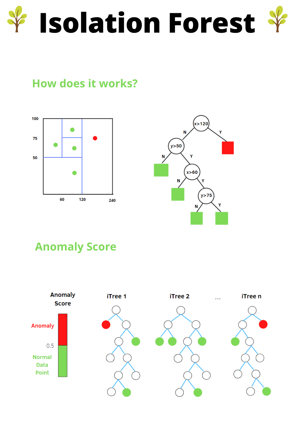
Figure 3: Anomaly detection with isolation forest better programming – Artofit Since real data can be hard and expensive to obtain, synthetic data generation has become instrumental in validating modern detection approaches. Building upon foundational work in dataset generation [ 10 ] , researchers have developed increasingly sophisticated evaluation frameworks. The introduction of Deep Sets [ 28 ] provided crucial tools for analyzing more complex security events, while new techniques [ 1 ] address the challenges of high-dimensional, sparse data environments.
This section describes the data processing and machine learning methods used to detect anomalies in network scan data. We first discuss the structure of the data as it determines the type of data preprocessing required. Then we describe two feature engineering methods that we use as well as the new siForest algorithm and its implementation. Censys is a company and internet intelligence platform designed to index and analyze data gathered from continuous, large-scale scans of the internet. For the entire public IPv4 address space, it scans for all available IP and port combinations with automated protocol identification. This process produces a precise snapshots of the current state of the internet. A typical dataset consists of a set of scans and each scan includes an IPv4 address, which is the unique identifier of the scanned device, a list of services–applications or protocols available on the device, and a list of the corresponding network ports.
This dataset is categorical, consisting primarily of lists. Moreover, objects in the lists are discrete values such as IP addresses, protocol names, and port numbers. To prepare it for machine learning analysis, it needs to undergo preprocessing steps. Established preprocessing strategies for categorical data aim to balance the trade-off between preserving important information and reducing the complexity of the data [ 30 ] . Next we describe two methods suitable for our data and discuss their advantages and drawbacks.
The flattened-data approach restructures network scan data by converting lists of ports and their associated services for each IP address into individual rows, creating a granular representation of IP-port-service combinations. Each row in the transformed dataset corresponds to a unique combination of an IP address, a port, and a service, with services converted into unique integer identifiers for efficient processing. This transformation represents in each row a single port and its corresponding service for a given IP.
For example, a scan originally represented by one row with a list of ports and services is expanded into multiple rows, with each row representing a specific port-service pair for that scan. The flattening approach avoids the feature explosion associated with one-hot encoding while maintaining the relationships between IPs, ports, and services. The transformation can increase the number of rows of the dataset. For instance, transforming data for 100 IPs, 100 scans average per IP, and each scan with an average of 10 ports and 10 corresponding services, generates approximately 100,000 rows, while the raw data has only 10,000 rows. However, this 10-fold increase results from reformatting through unfolding of one list feature into 10 simple (integer) ones, not from computational inefficiency. The main drawback of this method is that, while we need to identify anomalous IPs, the rows in this representation correspond to scans rather than IPs.
The summarization approach aggregates the data to create a fixed-length feature vector for every IP. The method restructures the data into a data frame with a row for each IP address, where each port and service is represented as a separate column, and the values provide the number of times the corresponding port or service are used for that IP. While this approach reduces the number of rows (data points) required, it leads to a large number of columns. Since the number of possible services and ports of Censys data are currently 116 and 3552, respectively, the number of features could go up to more than 3600, even if a much smaller number of them are used per individual IP address. With such a high number of features, the risk of feature sparsity and overfitting increases. Another drawback of this approach is that it doesn’t capture the correspondence between services and ports. While we do represent which ports and which services are used per IP, we don’t encode how they match to each other. This can be avoided by having all possible pairs (service, port) as features, but that will further increase the number of features by two orders of magnitude and will further exacerbate the problem.
Figure 2 shows comparison between the number of datapoints and features of the above methods compared to those for the original dataset used in our experiments. In network scan data, where features such as ports and services are represented as lists tied to IP addresses, retaining the structure of the data is essential. The proposed modification of the iForest algorithm addresses the limitations of the original algorithm to work with such structured data. The core idea of the proposed method, siForest, is to halt further tree partitioning when all data points in a leaf node belong to the same IP address. The design ensures that related data points, such as the ports and services associated with an IP, remain grouped together, preserving their contextual relationships.
This process is illustrated in Figure 3 , which shows three decision trees representing the different approaches considered in this paper. The first tree illustrates using iForest combined with the flattening method, which keeps the number of features low but does not allow the algorithm to identify anomalous IPs, as it operates at the scan level. The second tree, using the summarization method, aggregates scans into single IP-level data points, but this drastically increases the number of features and reduces the model’s efficacy. The third tree demonstrates the siForest approach, which uses scans as data points but stops splitting when a node contains only scans from the same IP. This maintains a low number of features while allowing it to detect anomalies at the IP level. It combines the advantages of the other two methods without their respective drawbacks.
To adapt the iForest algorithm for set-structured data, we made several updates to the original scikit-learn implementation [ 24 ] . The most significant change is in the tree construction process, where siForest implements a stopping condition based on IP groupings. In the original iForest, partitioning continues until each leaf contains a single data point. However, siForest halts partitioning once all data points in a node belong to the same IP address, regardless of the number of the data points at the leaf.
This adjustment modifies the tree-building logic to evaluate whether all data points in a node share the same IP during splits. Additionally, the leaf structure is updated to store IP-specific data. This preserves the relationships between ports and services and the IP address they belong to, which are critical for detecting anomalies at IP level. Another important update involves the scoring mechanism. Unlike the original implementation, where anomaly scores are calculated for individual data points, siForest aggregates scores at the IP level. We introduce two aggregation strategies: one that uses the minimum anomaly score among all scans for an IP and another using the average score. This allows siForest to capture both extreme outliers and persistent anomalous behavior.
In this section, we describe our procedure for comparing the performances of the different implementations of Isolation Forest described above and discuss the results. We evaluated siForest against the traditional iForest algorithm using synthetic datasets that mirror real-world network traffic patterns. The datasets combine normal service-port pairings based on typical network scans with controlled anomalies to test detection capabilities under various configurations and preprocessing strategies. For data preprocessing, standard python libraries numpy [ 15 ] and pandas [ 23 ] are used.
2. System Architecture & Core Working Principles To create a realistic testing environment, the synthetic data incorporates both normal behavior and injected anomalies. Normal patterns reflect common service-port combinations observed in network scans, while anomalies include usage spikes, non-standard port assignments, and service-port mismatches. This controlled environment enables consistent testing across scenarios.
We compare the three methods discussed in Section 3.2 to address the set-structured nature of network scan data. We use the implementation of iForest on scikit-learn package [ 24 ] and our implementation of siForest as described above. Both algorithms use the same number of 100 estimators (trees) for consistency. We calculate anomaly scores at the IP level using the minimum score option as it gives a better performance for the generated data.
Data is generated for each of the two anomaly types, with 10 different random sets for each type. The three tested algorithms are then run on the same data, and their predictions are compared with the known (planted) anomalies. Performance is evaluated using standard metrics such as precision, recall, and F2-score. Although precision and F2-score provide valuable information that should be taken into account, recall is most relevant because attack surface identification primarily aims to avoid missing potential vulnerabilities. Detected anomalies are inspected by a human expert to determine if they may pose a real threat. However, if a vulnerability is missed by the anomaly detector, it will never be analyzed or addressed.
While trying to mimic Censys [ 6 ] collected network data, our study uses synthetic dataset to enable controlled testing of anomaly detection methods. We base normal network behavior on common service-port combinations documented in Censys, such as HTTP on port 80 and FTP on port 21. A Python dictionary stores these standard mappings to maintain consistency in generating baseline network activity.
A synthetic data approach allows precise injection of anomalies through deviations from expected service-port relationships. The evaluation covers two distinct anomaly classes, described below, to test how each method’s detection capabilities vary depending on the anomaly type. This design choice overcomes the limitation of unlabeled anomalies in raw Censys data while allowing flexibility in defining both ”normal” and ”anomalous” activity [ 4 ] .
Our evaluation incorporates two distinct anomaly patterns in the synthetic dataset. The first type, referred to as anomaly type 1, represents sudden usage spikes, where an IP address shows unexpected activity across one or more ports [ 7 ] . Such patterns often indicate network scanning or denial-of-service attempts. Figure 4 shows these volume-based anomalies, with red bars marking abnormal scanning activity against the blue baseline.
The second type, referred to as anomaly type 2, introduces non-standard service-port combinations [ 13 ] , such as HTTP services running on unexpected ports. Figure 5 illustrates these configuration anomalies, with red segments showing services on non-standard ports. By generating these irregular pairings, the dataset evaluates the model’s capability to detect anomalies that arise from misconfigurations or intentional misuse of network resources.
The frequency and intensity of both anomaly types can be adjusted using tunable parameters to create diverse testing scenarios, from subtle deviations to clear outliers, enabling a thorough assessment of each model’s detection sensitivity across different anomaly distributions. The evaluation results, shown on Figure 6 , reveal distinct performance patterns across anomaly types and detection methods. For type 1 anomalies (usage spikes), siForest demonstrated robust performance with a precision of 0.285, recall of 0.520, and F2-score of 0.435. This balanced detection capability suggests the method effectively identifies volume-based anomalies while maintaining reasonable false positive rates.
The flattening preprocessing approach, implemented through iForest Pairs, shows significant limitations with type 1 anomalies. Its precision (0.060), recall (0.220), and F2-score (0.131) are substantially lower than the other methods, likely due to the loss of structural information during the flattening process. In contrast, iForest with summarization preprocessing achieved the highest precision (0.61) among all approaches while maintaining strong recall (0.58), resulting in an F2-score of 0.59. This performance indicates that summarization effectively preserves critical patterns for type 1 anomalies. It seems the summarized data approach successfully captures unusual behavior for type 1 anomalies because it aggregates and counts occurrences, aligning with the volume-based nature of this anomaly type characterized by increased usage patterns.
For type 2 anomalies (unusual port usage), iForest Summarization struggles, achieving only 0.027 precision, 0.100 recall, and an F2-score of 0.060. This sharp decline in performance suggests that the summarization strategy is particularly ineffective for detecting this type of anomaly. In comparison, Custom iForest demonstrates the strongest performance for type 2 anomalies, with a precision of 0.404, recall of 0.709, and F2-score of 0.599. These results, particularly the high recall, suggest the method excels at identifying structural anomalies in service-port relationships.
The flattening approach (iForest pairs) shows better performance for type 2 anomalies compared to type 1, with a precision of 0.427, recall of 0.336, and F2-score of 0.344. While still underperforming compared to Custom iForest, this approach demonstrates less dramatic degradation compared to its performance on type 1 anomalies. The two plots reveal distinct performance characteristics across different preprocessing strategies. Summarization preprocessing dominates in precision for type 1 anomalies but performs poorly for type 2 anomalies. Custom iForest (siForest) achieves consistently good performance across both anomaly types – it shows the best overall performance for type 2 anomalies and maintains strong results for type 1 anomalies, particularly in recall.
This paper discusses the usage of the Isolation forest approach to detecting anomalies in internet scan data for applications in attack surface identification. We are applying two data preprocessing methods and also develop a modification of the standard iForest algorithm that is able to work with a set-structured data. Our analysis shows that the effectiveness of the methods depend on the type of anomaly being present. While the summarization method particularly excels at identifying volume-based anomalies, it performs poorly when detecting unusual port usage patterns. The flattening approach, on the other hand, performs poorly on volume-based anomalies, but beats the summarization one for anomalies based on unusual port usage.
The proposed siForest algorithm demonstrates the most consistent performance across both anomaly types. For unusual port usage, it achieves the best overall performance, while for the other type of anomaly its performance comes close to that of the summarization approach, especially with respect to the important recall metrics. These results suggest that proper preprocessing methods can help detect anomalies in set-structured datasets such as ones based on Censys internet scans, but siForest is the only methods among the tested ones that shows consistently good performance over all anomaly types.
This work leaves several open avenues for future research. One is to test the algorithms on more anomaly types and on datasets of varying sizes. Applying siForest to real-world datasets is also very interesting although such data may be hard to obtain. Integrating graph-based techniques to capture more intricate relationships within network data is another promising direction, as is the development of automated mechanisms for anomaly characterization [ 8 ] .
By broadening its scope and improving its scalability, SiForest has the potential to develop into a practical tool for anomaly detection in set-structured data, and in cybersecurity and attack surface identification, in particular. Anomaly detection is vital across industries, revealing outliers in data that signal problems or unique insights. Isolation Forests offer a powerful solution, isolating anomalies from normal data. In this tutorial, we will explore the Isolation Forest algorithm's implementation for anomaly detection using the Iris flower dataset, showcasing its effectiveness in identifying outliers amidst multidimensional data.
Anomalies , also known as outliers, are data points that deviate significantly from the expected behavior or norm within a dataset. They are crucial to identify because they can signal potential problems, fraudulent activities, or interesting discoveries. Anomaly detection plays a vital role in various fields, including data analysis, machine learning, and network security.
There are essentially three types of anomalies: point anomalies, contextual anomalies, and collective anomalies. Isolation Forest is an unsupervised anomaly detection algorithm particularly effective for high-dimensional data. It operates under the principle that anomalies are rare and distinct, making them easier to isolate from the rest of the data. Unlike other methods that profile normal data, Isolation Forests focus on isolating anomalies. At its core, the Isolation Forest algorithm, it banks on the fundamental concept that anomalies, they deviate significantly, thereby making them easier to identify.
Isolation Forests excel at anomaly detection by leveraging a unique approach: isolating anomalies instead of profiling normal data points. The workings of isolation forests are defined below: Let's see implementation for Isolation Forest algorithm for anomaly detection using the Iris flower dataset from scikit-learn. In the context of the Iris flower dataset, the outliers would be data points that do not correspond to any of the three known Iris flower species (Iris Setosa, Iris Versicolor, and Iris Virginica). The following steps are mentioned: This code creates an Isolation Forest classifier instance using the IsolationForest class. C ontamination is a parameter that specifies the expected proportion of anomalies in the data. Here, it's set to 0.1 (10%).
The predict method returns labels indicating whether each data point is classified as normal (1) or anomalous (-1) by the model. The distribution of the anomalies in the training data is different from the distribution of the anomalies in the test data. In the training data, the anomalies tend to be located on the edges of the plot. In the test data, the anomalies are more scattered throughout the plot.
3. Software Implementation, Frameworks & Protocols The Isolation Forest algorithm offers an efficient solution for identifying anomalies, especially in datasets with multiple dimensions. It stands out by isolating outliers rather than profiling normal cases, making it more adept at uncovering rare instances that differ from the usual pattern.
Get paid to write technical tutorials and select a tech-focused charity to receive a matching donation. The Wave has everything you need to know about building a business, from raising funding to marketing your product. From GPU-powered inference and Kubernetes to managed databases and storage, get everything you need to build, scale, and deploy intelligent applications.
Anomaly detection is crucial in data mining and machine learning, finding applications in fraud detection, network security, and more. The Isolation Forest algorithm, introduced by Fei Tony Liu and Zhi-Hua Zhou in 2008, stands out among anomaly detection methods. It uses decision trees to efficiently isolate anomalies by randomly selecting features and splitting data based on threshold values. This approach is effective in quickly identifying outliers, making it well-suited for large datasets where anomalies are rare and distinct.
As in this article, we delve into the workings of the Isolation Forest algorithm, its implementation in Python , and its role as a powerful tool in anomaly detection. We also explore the metrics used to evaluate its performance and discuss its applications across various domains. In this article, you will get a clear understanding of the Isolation Forest algorithm in Python. We will look at how to use Isolation Forest for finding outliers in data. You will learn about the Isolation Forest Python library and see an easy Isolation Forest example. By the end, you will know how to use isolation forest outlier detection in your own projects.
Isolation Forest is a method used to find unusual data points, known as anomalies or outliers, in a dataset. It is particularly good at spotting these anomalies in large amounts of data. Since its introduction, Isolation Forest has gained popularity as a fast and reliable algorithm for anomaly detection in various fields such as cybersecurity, finance, and medical research.
Isolation Forests(IF), similar to Random Forests , are build based on decision trees . And since there are no pre-defined labels here, it is an unsupervised model. Isolation Forests were built based on the fact that anomalies are the data points that are “few and different”. In an Isolation Forest, randomly sub-sampled data is processed in a tree structure based on randomly selected features. The samples that travel deeper into the tree are less likely to be anomalies as they required more cuts to isolate them. Similarly, the samples which end up in shorter branches indicate anomalies as it was easier for the tree to separate them from other observations.
As mentioned earlier, Isolation Forests outlier detection are nothing but an ensemble of binary decision trees. And each tree in an Isolation Forest is called an Isolation Tree(iTree). The algorithm starts with the training of the data, by generating Isolation Trees. After creating an ensemble of iTrees (Isolation Forest), the model training is complete. During scoring, the system traverses each data point through all the previously trained trees. The model assigns an ‘anomaly score’ to each data point based on the depth of the tree needed to reach that point. This score aggregates the depths obtained from each of the iTrees. An anomaly score of -1 assigns anomalies and 1 to normal points based on the contamination parameter (percentage of anomalies present in the data).
Source: IEEE . We can see that it was easier to isolate an anomaly compared to a normal observation. You can take a look at Isolation Forest documentation in sklearn to understand the model parameters. Isolation Forests are computationally efficient and researchers have proven them to be very effective in anomaly detection. Despite its advantages, there are a few limitations as mentioned below.
Well, to understand the second point, we can take a look at the below anomaly score map. Here, in the score map on the right, we can observe that the points in the center obtained the lowest anomaly score, as expected. However, we can see four rectangular regions around the circle with lower anomaly scores as well. So, when scoring a new data point in any of these rectangular regions, it might not detect it as an anomaly.
Similarly, in the above figure, we can see that the model resulted in two additional blobs(on the top right and bottom left ) which never even existed in the data. Whenever a node splits in an iTree based on a threshold value, it divides the data into left and right branches, resulting in horizontal and vertical branch cuts. And these branch cuts result in this model bias.
The above figure shows branch cuts after combining outputs of all the trees of an Isolation Forest. Here, we can observe how the rectangular regions with lower anomaly scores formed in the left figure. And also the right figure shows the formation of two additional blobs due to more branch cuts. To overcome this limit, an extension to Isolation Forests called ‘Extended Isolation Forests’ was introduced by Sahand Hariri .
In EIF, horizontal and vertical cuts were replaced with cuts with random slopes. Despite introducing EIF (Extended Isolation Forest), the use of Isolation Forests for anomaly detection remains widespread across various fields. The Local Outlier Factor (LOF) algorithm is a powerful tool for detecting anomalies in data by evaluating the density of points relative to their neighbors. Unlike traditional anomaly detection methods, LOF does not require assuming a specific data distribution, making it suitable for a wide range of applications. When implementing LOF, setting the n_estimators parameter appropriately ensures robust performance, balancing computational efficiency with detection accuracy. It is important to note that LOF performs well with both normal and anomalous instances, as it identifies points that deviate significantly from their local neighborhood.
Hope you like the isolation forest example, which demonstrates the isolation forest anomaly detection algorithm in Python. The isolation forest is a powerful tool for identifying anomalies in complex datasets. By applying the isolation forest anomaly detection method, you can isolate outliers and gain valuable insights from your data. The isolation forest algorithm is a highly effective solution for various applications that require anomaly detection.
By leveraging random partitioning and regression techniques, LOF achieves scalable and efficient anomaly detection, even with large datasets. Adjusting the sampling size parameter enables fine-tuning of the algorithm to suit specific data characteristics, ensuring optimal results in real-world applications. A. Random Forest is a supervised learning algorithm for classification and regression tasks using decision trees. Isolation Forest is an unsupervised algorithm for anomaly detection, isolating anomalies based on unique properties.
4. Practical Deployment, Analysis & Case Studies A. Isolation Forest works by randomly selecting a feature from the dataset and a split value to create partitions of the data. The process repeats recursively until it isolates anomalies in their own partitions. Isolation Forest quickly finds outliers by randomly splitting data. Works well on large datasets but needs the right number of expected outliers.
Isolation Forest doesn’t measure distance. It finds outliers by seeing how quickly it can isolate data points. Points that are easy to isolate are likely outliers. The media shown in this article are not owned by Analytics Vidhya and are used at the Author’s discretion. This is a great blog post! I'm a big fan of using Isolation Forest for anomaly detection.
This is a great blog post! I'm a big fan of using Isolation Forest for anomaly detection. The IsolationForest ‘isolates’ observations by randomly selecting a feature and then randomly selecting a split value between the maximum and minimum values of the selected feature. Since recursive partitioning can be represented by a tree structure, the number of splittings required to isolate a sample is equivalent to the path length from the root node to the terminating node.
This path length, averaged over a forest of such random trees, is a measure of normality and our decision function. Random partitioning produces noticeably shorter paths for anomalies. Hence, when a forest of random trees collectively produce shorter path lengths for particular samples, they are highly likely to be anomalies. If max_samples is larger than the number of samples provided, all samples will be used for all trees (no sampling).
The amount of contamination of the data set, i.e. the proportion of outliers in the data set. Used when fitting to define the threshold on the scores of the samples. Changed in version 0.22: The default value of contamination changed from 0.1 to 'auto' . Note: using a float number less than 1.0 or integer less than number of features will enable feature subsampling and leads to a longer runtime.
If True, individual trees are fit on random subsets of the training data sampled with replacement. If False, sampling without replacement is performed. The number of jobs to run in parallel for fit . None means 1 unless in a joblib.parallel_backend context. -1 means using all processors. See Glossary for more details.
Controls the pseudo-randomness of the selection of the feature and split values for each branching step and each tree in the forest. When set to True , reuse the solution of the previous call to fit and add more estimators to the ensemble, otherwise, just fit a whole new forest. See the Glossary .
Offset used to define the decision function from the raw scores. We have the relation: decision_function = score_samples - offset_ . offset_ is defined as follows. When the contamination parameter is set to “auto”, the offset is equal to -0.5 as the scores of inliers are close to 0 and the scores of outliers are close to -1. When a contamination parameter different than “auto” is provided, the offset is defined in such a way we obtain the expected number of outliers (samples with decision function < 0) in training.
Names of features seen during fit . Defined only when X has feature names that are all strings. Unsupervised Outlier Detection. Estimate the support of a high-dimensional distribution. The implementation is based on libsvm. The implementation is based on an ensemble of ExtraTreeRegressor. The maximum depth of each tree is set to ceil(log_2(n)) where \(n\) is the number of samples used to build the tree (see [1] for more details).
F. T. Liu, K. M. Ting and Z. -H. Zhou. “Isolation forest.” 2008 Eighth IEEE International Conference on Data Mining (ICDM), 2008, pp. 413-422. F. T. Liu, K. M. Ting and Z. -H. Zhou. “Isolation-based anomaly detection.” ACM Transactions on Knowledge Discovery from Data (TKDD) 6.1 (2012): 1-39.
For an example of using isolation forest for anomaly detection see IsolationForest example . The anomaly score of an input sample is computed as the mean anomaly score of the trees in the forest. The measure of normality of an observation given a tree is the depth of the leaf containing this observation, which is equivalent to the number of splittings required to isolate this point. In case of several observations n_left in the leaf, the average path length of an n_left samples isolation tree is added.
The input samples. Internally, it will be converted to dtype=np.float32 and if a sparse matrix is provided to a sparse csr_matrix . 5. Performance Evaluation & Extended Technical Observations The anomaly score of the input samples. The lower, the more abnormal. Negative scores represent outliers, positive scores represent inliers.
The decision_function method can be parallelized by setting a joblib context. This inherently does NOT use the n_jobs parameter initialized in the class, which is used during fit . This is because, calculating the score may actually be faster without parallelization for a small number of samples, such as for 1000 samples or less. The user can set the number of jobs in the joblib context to control the number of parallel jobs.
The input samples. Use dtype=np.float32 for maximum efficiency. Sparse matrices are also supported, use sparse csc_matrix for maximum efficiency. If True, will return the parameters for this estimator and contained subobjects that are estimators. The input samples. Internally, it will be converted to dtype=np.float32 and if a sparse matrix is provided to a sparse csr_matrix .
For each observation, tells whether or not (+1 or -1) it should be considered as an inlier according to the fitted model. The predict method can be parallelized by setting a joblib context. This inherently does NOT use the n_jobs parameter initialized in the class, which is used during fit . This is because, predict may actually be faster without parallelization for a small number of samples, such as for 1000 samples or less. The user can set the number of jobs in the joblib context to control the number of parallel jobs.
The anomaly score of an input sample is computed as the mean anomaly score of the trees in the forest. The measure of normality of an observation given a tree is the depth of the leaf containing this observation, which is equivalent to the number of splittings required to isolate this point. In case of several observations n_left in the leaf, the average path length of an n_left samples isolation tree is added.
The score function method can be parallelized by setting a joblib context. This inherently does NOT use the n_jobs parameter initialized in the class, which is used during fit . This is because, calculating the score may actually be faster without parallelization for a small number of samples, such as for 1000 samples or less. The user can set the number of jobs in the joblib context to control the number of parallel jobs.
Note that this method is only relevant when this estimator is used as a sub-estimator within a meta-estimator and metadata routing is enabled with enable_metadata_routing=True (see sklearn.set_config ). Please check the User Guide on how the routing mechanism works. True : metadata is requested, and passed to fit if provided. The request is ignored if metadata is not provided.
None : metadata is not requested, and the meta-estimator will raise an error if the user provides it. str : metadata should be passed to the meta-estimator with this given alias instead of the original name. The default ( sklearn.utils.metadata_routing.UNCHANGED ) retains the existing request. This allows you to change the request for some parameters and not others.
The method works on simple estimators as well as on nested objects (such as Pipeline ). The latter have parameters of the form
Project Overview This repository provides an end-to-end solution for detecting anomalies in network traffic using a hybrid approach. The first step utilizes the Isolation Forest algorithm for unsupervised anomaly detection, followed by a deep learning neural network for binary classification of normal and anomalous data. The system includes data preprocessing, feature engineering, model training, and evaluation, offering a comprehensive pipeline for anomaly detection tasks.
Min-Max scaling of numerical features to ensure all features are on the same scale. Feature engineering by creating additional features like TotalBytes and TotalPackets. Anomaly Detection with Isolation Forest: An Isolation Forest model is trained on the features to detect anomalies in the dataset. The predicted anomalies are labeled and used to train the deep learning model. Deep Learning Model: A simple neural network model is constructed using Keras with two hidden layers (64 and 32 neurons). The model is compiled using binary cross-entropy loss and Adam optimizer, and trained on the labeled data. Predictions are evaluated using metrics such as confusion matrix, classification report, and ROC-AUC.
Confusion Matrix: Provides insights into true positives, true negatives, false positives, and false negatives. Classification Report: Includes precision, recall, F1-score, and support for both normal and anomalous classes. ROC Curve and AUC: Plots the ROC curve and calculates the Area Under the Curve (AUC), which indicates the model’s ability to distinguish between normal and anomalous traffic.
Confusion Matrix: Visualizes the classification performance. Classification Report: Shows the precision, recall, and F1-score for each class. ROC-AUC: The AUC score indicates how well the model differentiates between normal and anomalous traffic. The dataset used in this project is a synthetic network traffic dataset, which includes various features such as BytesSent , BytesReceived , PacketsSent , PacketsReceived , and Duration . The target variable, IsAnomaly , indicates whether a traffic instance is an anomaly (1) or normal (0).
To run the code and experiment with the anomaly detection pipeline, you need to have the following libraries installed: This project implements an anomaly detection system for synthetic network traffic data using a combination of an Isolation Forest model and a deep learning neural network. The system is designed to identify anomalies in network traffic, which may indicate potential security threats or unusual activity.
This project implements an anomaly detection system for monitoring network performance. Using simulated network data, the system employs the Isolation Forest machine learning algorithm to detect anomalies (outliers) such as sudden spikes in latency, signal strength fluctuations, packet loss, and interference. The system also supports real-time anomaly detection and provides model evaluation metrics.
The main script for training the anomaly detection model is located in the src/anomaly_detection.py file. You can run it directly using: Harvested Online Documentation & Reference Sources • https://arxiv.org/html/2412.06015v1 • https://www.geeksforgeeks.org/machine-learning/anomaly-detection-using-isolation-forest/ • https://www.digitalocean.com/community/tutorials/anomaly-detection-isolation-forest • https://www.analyticsvidhya.com/blog/2021/07/anomaly-detection-using-isolation-forest-a-complete-guide/ • https://scikit-learn.org/stable/modules/generated/sklearn.ensemble.IsolationForest.html • https://github.com/MahmoudAbuAwd/Anomaly-Detection-in-Network-Traffic-Using-Isolation-Forest-and-Deep-Learning • https://github.com/ameekbains/Network-Anomaly-Detection
Extracted Research Figures & Simulation Topologies
Total 3 diagrams and telemetry visual outputs extracted directly from the complete technical documentation.
Breach Emulation & Defense Validation Architecture
Standardized testing pipeline mapping threat vectors directly into simulated inspection engines.
(AttackIQ / SafeBreach)
(Burp Suite Pro)
(Cisco Packet Tracer)
(Metasploit Engine)
(KnowBe4 Training)
Sample Simulation Code & Telemetry Log
Automated tool orchestration script and command window outputs for Network Anomaly Detection Using Isolation Forest Algorithm.
! Define Extended Access List to Block Malicious Traffic ip access-list extended SECURE_PERIMETER_ACL remark Block Inbound Telnet and Unencrypted Services deny tcp any any eq 23 log remark Permit Verified Web SSL Traffic permit tcp any any eq 443 permit tcp any any eq 80 remark Mitigate ICMP Flood and Ping Sweeps permit icmp any any echo-reply deny icmp any any echo log deny ip any any log
! Apply ACL to Ingress Interface GigabitEthernet0/0 interface GigabitEthernet0/0 ip access-group SECURE_PERIMETER_ACL in no shutdown end write memory
Extended IP access list SECURE_PERIMETER_ACL (Cisco Packet Tracer) ──────────────────────────────────────────────────────────────────────── 10 deny tcp any any eq telnet log (142 matches) [Probes Dropped] 20 permit tcp any any eq 443 (18402 matches) [TLS 1.3 Traffic Permitted] 30 permit tcp any any eq 80 (4812 matches) 40 deny icmp any any echo log (524 matches) [Flood Mitigated] 50 deny ip any any log (38 matches) [Default Implicit Deny Rule] ──────────────────────────────────────────────────────────────────────── [✓] Packet Tracer Verification: 0 Unsanitized Ingress Leaks on Gi0/0
| Interface Port | Network Zone | Filter Applied | Traffic Processed | Firewall Decision |
|---|---|---|---|---|
| Gig0/0 (WAN) | Untrusted External | Extended ACL 101 | 24,810 Packets | INSPECTED & FILTERED |
| Gig0/1 (DMZ) | Public Web Services | Port 443 Only | 18,402 Packets | PERMITTED |
| Gig0/2 (LAN) | Corporate Users | 802.1X Port Security | 142 Probes | DENIED & QUARANTINED |