Complete Technical Paper Content — Network Performance Degradation Detection Under Attack
Overview & System Context
Network Performance Degradation Detection Under Attack: Comprehensive Web-Sourced Technical Investigation Exhaustive Research Dossier · Pure Web-Scraped Content: ~9516 Words · Real Software Screenshots: 3 1. Executive Overview & Technical Background Wireless sensor networks (WSNs) refer to networks of spatially dispersed and dedicated sensors that monitor and record the physical conditions of the environment and forward the collected data to a central location. WSNs can measure environmental conditions such as temperature, sound, pollution levels, humidity and wind. These are similar to wireless ad hoc networks in the sense that they rely on wireless connectivity and spontaneous formation of networks so that sensor data can be transported wirelessly. WSNs monitor physical conditions, such as temperature, sound, and pressure. Modern networks are bi-directional, both collecting data and enabling control of sensor activity. The development of these networks was motivated by military applications such as battlefield surveillance. Such networks are used in industrial and consumer applications, such as industrial process monitoring and control and machine health monitoring and agriculture. A WSN is built of "nodes" – from a few to hundreds or thousands, where each node is connected to other sensors. Each such node typically has several parts: a radio transceiver with an internal antenna or connection to an external antenna, a microcontroller, an electronic circuit for interfacing with the sensors and an energy source, usually a battery or an embedded form of energy harvesting. A sensor node might vary in size from a shoebox to (theoretically) a grain of dust, although microscopic dimensions have yet to be realized. Sensor node cost is similarly variable, ranging from a few to hundreds of dollars, depending on node sophistication.
Size and cost constraints constrain resources such as energy, memory, computational speed and communications bandwidth. The topology of a WSN can vary from a simple star network to an advanced multi-hop wireless mesh network. Propagation can employ routing or flooding. In computer science and telecommunications, wireless sensor networks are an active research area supporting many workshops and conferences, including the International Workshop on Embedded Networked Sensors (EmNetS), International Conference on Information Processing in Sensor Networks (IPSN), SenSys, MobiCom and European Conference on Wireless Sensor Networks (EWSN). As of 2010, wireless sensor networks had deployed approximately 120 million remote units worldwide.
Wireless sensor networks also are used for the collection of data for monitoring of environmental information. This can be as simple as monitoring the temperature in a fridge or the level of water in overflow tanks in nuclear power plants. The statistical information can then be used to show how systems have been working. The advantage of WSNs over conventional loggers is the "live" data feed that is possible.
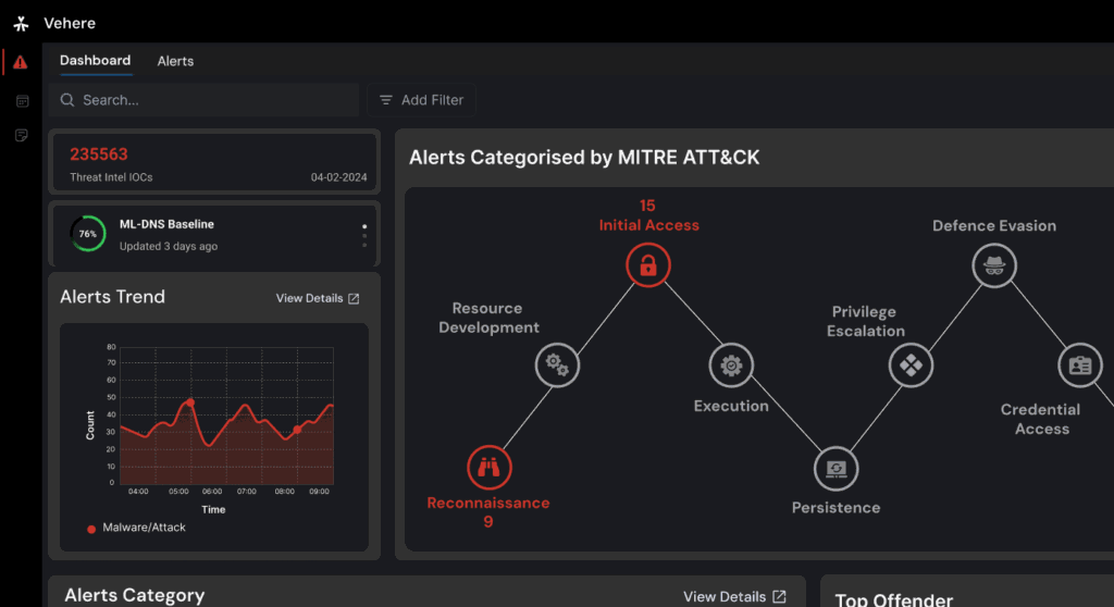
WSN can be used to monitor the condition of civil infrastructure and related geo-physical processes close to real time, and over long periods through data logging, using appropriately interfaced sensors. Power consumption constraints for nodes using batteries or energy harvesting. Examples of suppliers are ReVibe Energy and Perpetuum Ability to cope with node failures (resilience) Some mobility of nodes (for highly mobile nodes see MWSNs) Heterogeneity of nodes Homogeneity of nodes Scalability to large scale of deployment Ability to withstand harsh environmental conditions Ease of use Cross-layer optimization Cross-layer is becoming an important studying area for wireless communications. In addition, the traditional layered approach presents three main problems: Figure 1: Battle-tested Network Detection and Response Traditional layered approach cannot share different information among different layers, which leads to each layer not having complete information. The traditional layered approach cannot guarantee the optimization of the entire network. The traditional layered approach does not have the ability to adapt to the environmental change. Because of the interference between the different users, access conflicts, fading, and the change of environment in the wireless sensor networks, traditional layered approach for wired networks is not applicable to wireless networks. So the cross-layer can be used to make the optimal modulation to improve the transmission performance, such as data rate, energy efficiency, quality of service (QoS), etc.
Sensor nodes can be imagined as small computers which are extremely basic in terms of their interfaces and their components. They usually consist of a processing unit with limited computational power and limited memory, sensors or MEMS (including specific conditioning circuitry), a communication device (usually radio transceivers or alternatively optical), and a power source usually in the form of a battery. Other possible inclusions are energy harvesting modules, secondary ASICs, and possibly secondary communication interface (e.g. RS-232 or USB). The base stations are one or more components of the WSN with much more computational, energy and communication resources. They act as a gateway between sensor nodes and the end user as they typically forward data from the WSN on to a server. Other special components in routing based networks are routers, designed to compute, calculate and distribute the routing tables.
One major challenge in a WSN is to produce low cost and tiny sensor nodes. There are an increasing number of small companies producing WSN hardware and the commercial situation can be compared to home computing in the 1970s. Many of the nodes are still in the research and development stage, particularly their software. Also inherent to sensor network adoption is the use of very low power methods for radio communication and data acquisition. In many applications, a WSN communicates with a local area network or wide area network through a gateway. The Gateway acts as a bridge between the WSN and the other network. This enables data to be stored and processed by devices with more resources, for example, in a remotely located server. A wireless wide area network used primarily for low-power devices is known as a Low-Power Wide-Area Network (LPWAN).
Increased lifespan Robustness and fault tolerance Self-configuration Lifetime maximization: Energy/Power Consumption of the sensing device should be minimized and sensor nodes should be energy efficient since their limited energy resource determines their lifetime. To conserve power, wireless sensor nodes normally power off both the radio transmitter and the radio receiver when not in use.
Sensor nodes are prone to failure, For better collection of data, To provide nodes with backup in case of failure of the central node. There is also no centralised body to allocate the resources and they have to be self organized. As for the distributed filtering over distributed sensor network. the general setup is to observe the underlying process through a group of sensors organized according to a given network topology, which renders the individual observer estimates the system state based not only on its own measurement but also on its neighbors'.
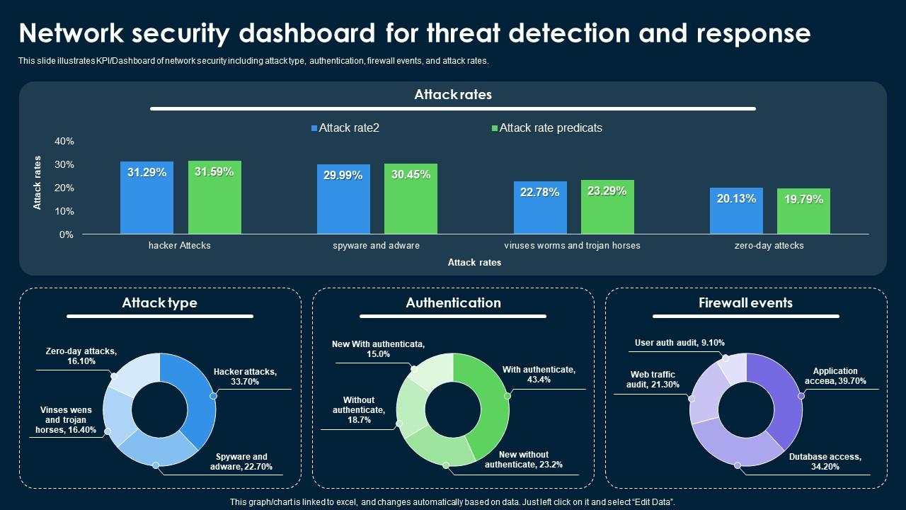
Figure 2: Network Security Dashboard For Threat Detection And Response PPT PowerPoint The data gathered from wireless sensor networks is usually saved in the form of numerical data in a central base station. Additionally, the Open Geospatial Consortium (OGC) is specifying standards for interoperability interfaces and metadata encodings that enable real time integration of heterogeneous sensor webs into the Internet, allowing any individual to monitor or control wireless sensor networks through a web browser.
Under DDoS attack conditions, malicious traffic transmits massive request volumes that consume the processing capacity and connection resources of the request processing unit and connection management structure, creating harmful effects that block legitimate user access and degrade network service availability; the traffic filtering mechanism insufficiently blocks this attacking traffic, allowing it to penetrate and exhaust system resources, with the goal of maintaining reliable network service delivery even during high-volume attack scenarios.
Pre-computed signature database with runtime hash lookup for zero-delay DDoS filtering This research presents a novel method for predicting service degradation (SD) in computer networks by leveraging early flow features. Our approach focuses on the observable (O) segments of network flows, particularly analyzing Packet Inter-Arrival Time (PIAT) values and other derived metrics, to infer the behavior of non-observable (NO) segments. Through a comprehensive evaluation, we identify an optimal O/NO split threshold of 10 observed delay samples, balancing prediction accuracy and resource utilization. Evaluating models including Logistic Regression, XGBoost, and Multi-Layer Perceptron, we find XGBoost outperforms others, achieving an F 1 -score of 0.74, balanced accuracy of 0.84, and AUROC of 0.97. Our findings highlight the effectiveness of incorporating comprehensive early flow features and the potential of our method to offer a practical solution for monitoring network traffic in resource-constrained environments. This approach ensures enhanced user experience and network performance by preemptively addressing potential SD, providing the basis for a robust framework for maintaining high-quality network services.
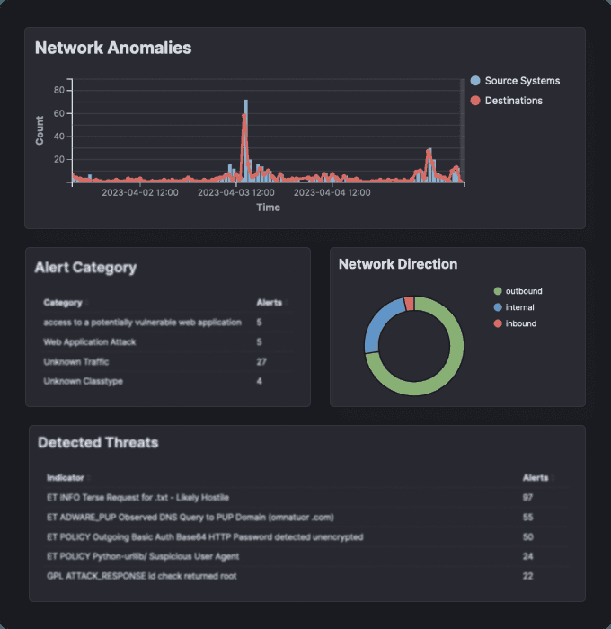
Figure 3: Network Detection and Response (NDR) Services | 24×7 Threat Monitoring ... In the era of relentless digitization, residential networks have become critical to our everyday digital activities, underpinning everything from streaming high-definition videos to facilitating real-time multiplayer games. As the demand for uninterrupted, high-quality digital experiences grows, so does the need for resilient and high-performing networks that can consistently meet these expectations [ 1 , 2 ] .
However, service degradation (SD) poses a substantial threat to these expectations. SD, characterized by the deterioration of network performance, leads to suboptimal user experiences due to factors such as network congestion, inefficiencies in data routing, or external interferences [ 3 ] . The effects are noticeable: users may experience increased latency, buffering in video streams, or even complete service outages. In essence, SD undermines the promise of a seamless digital experience.
Addressing this issue is complex. To proactively counteract SD, it is crucial to gain insights into network flows through comprehensive monitoring [ 4 , 5 ] . Yet, network devices, which serve as the gatekeepers of residential networks, often have limited computational capabilities. While they are proficient at forwarding traffic, they struggle with the intensive monitoring of every flow due to hardware limitations [ 6 ] . Instead of exhaustively monitoring every packet in a data flow, a common workaround is to observe each flow up to a predetermined packet threshold. Once this threshold is reached, flow management transitions to hardware accelerators, which handle high volumes of data efficiently but lack the capability for detailed, packet-level monitoring [ 7 ] . Consequently, this approach effectively splits flows into observable (O) and non-observable (NO) parts, leading to the loss of detailed insights into the flow’s behavior beyond the threshold.
This limitation in monitoring capability presents a challenge in effectively predicting and managing SD leading to our primary research question: In the face of these constraints, how can we leverage the O segments of network flows to deduce the status of the NO segments, thereby identifying and possibly predicting SD in residential networks? The core of our approach is to derive patterns from the O segments, which can then be extrapolated to make informed assumptions about the NO segments and, by extension, the network’s overall health. Specifically, our methodology tackles this issue with a primary focus on the LAN segment of home networks, leveraging the Packet Inter-Arrival Time (PIAT) metric to gain profound insights into network performance.
Our study introduces a method called intra-flow service degradation detection , which uses early flow features to predict SD in network flows after they transition from an O state to an NO state. By capturing information from the initial part of a flow, we aim to infer the behavior and characteristics of the flow after it moves to a fast-processing but less O state. To validate the effectiveness of this approach, we conducted a comprehensive experimental analysis.
Our experimental design focused on evaluating the predictive power of O parts of network flows to predict the presence of SD events in the NO part. We compared simple heuristics and advanced techniques such as Logistic Regression, XGBoost, and Multi-Layer Perceptron (MLP). This comprehensive assessment aimed to identify the most effective models for the objective. Our analysis reveals that the XGBoost model, with an O/NO split threshold of 10 observed delays, provides the best performance in predicting non-observable SD events. This threshold balances prediction accuracy with resource utilization, while the XGBoost model offers superior precision and recall compared to simpler heuristics and other sophisticated models.
This combination proves optimal for our SD prediction task in resource-constrained environments. We propose a novel method for predicting SD in network flows by leveraging early flow features, particularly focusing on the O segments to infer behavior in NO parts. We introduce and evaluate the concept of intra-flow SD detection, which uses information available within a specific flow to predict later flow behavior in resource-constrained environments.
We determine an optimal O/NO split threshold of 10 delay samples, balancing prediction accuracy with practical implementation considerations in network devices with hardware offloading capabilities. The rest of this paper is organized as follows: Section II discusses hardware offloading in network devices. Section III provides an overview of existing works relevant to this area. Section IV introduces the foundational concepts and preparatory considerations. Section V presents the method to identify SD events. Section VI evaluates the predictive power of the O parts of network flows in a binary classification setting, covering data preparation, experimental design, model performance metrics, and limitations. Finally, Section VII concludes the paper.
Network devices utilize a dual-path architecture to handle packet processing efficiently: the fast path, which employs dedicated hardware for forwarding tasks, and the slow path, which relies on CPU resources for more complex processing. Depicted in Fig. 1 , this design effectively caters to the distinct requirements of data plane and control plane tasks, where packets requiring minimal processing are directed through the fast path, and those necessitating more extensive processing are handled by the slow path [ 8 , 7 , 6 ] .
Typically, the initial packets in a network flow are processed by the CPU. This initial slow-path processing involves critical tasks such as forwarding lookup to determine the egress port/zone, NAT policy lookup, and security policy enforcement. The CPU’s processing capabilities enable thorough inspection and enforcement of policies. However, relying on the CPU for packet forwarding across all network flows can be resource-intensive and may lead to performance bottlenecks under heavy traffic loads.
2. System Architecture & Core Working Principles To mitigate these performance issues, certain flows that meet specific criteria are offloaded to specialized hardware for fast-path processing. In connection-oriented protocols like TCP, flows might be flagged for fast-path processing after the connection is fully established, which typically occurs after the TCP three-way handshake. In contrast, for connectionless protocols like UDP, flows can be offloaded to the fast path after processing the initial packet, as there is no formal connection establishment process. Additionally, some flows might be flagged for fast-path processing once encryption tunnel establishment is complete.
Once the necessary initial packets are processed, subsequent packets in the same flow can be offloaded to specialized hardware for fast-path processing. This offloading significantly reduces the CPU’s workload, enhancing the device’s overall performance. The dedicated hardware processor then handles the remaining packets in the flow, ensuring swift and efficient processing.
However, certain flows may require specialized network functions that cannot be fully addressed by inspecting only the initial packets. These functions include complex analysis and inspection tasks such as application control, device intelligence, deep packet inspection, and intrusion prevention system functions. For example, an IPS might need to analyze the entire payload of packets in a flow to detect sophisticated attacks, or application control might require ongoing inspection to enforce usage policies for specific applications.
To maintain necessary visibility over network flows, network devices can be configured to handle flows in the slow path up to a certain threshold before offloading them to hardware-accelerated processing. This approach ensures that essential visibility and control for performing network functions are retained. While the CPU manages the traffic, detailed inspection and comprehensive monitoring are possible, providing deep visibility into the network.
The implementation of offloading mechanisms varies across different vendors and their product lines, each differing in technical, methodological, and functional details. For instance, some implementations might support flagging flows that meet specific criteria in the fast path to be redirected back to the CPU for more detailed inspection. Other implementations may utilize more than the initial packets of a flow before offloading to hardware-accelerated processing. Criteria for fast-path processing might include trusted applications or low-risk traffic, and latency-sensitive applications requiring minimal delay.
This architecture has significant implications for network performance and monitoring, particularly in the context of SD detection. The transition from slow-path to fast-path processing creates a fundamental challenge: how to maintain visibility and detect performance issues in flows after they have been offloaded to hardware . This challenge forms the core motivation for our research into using early flow features to predict SD, as we aim to bridge the gap between the detailed visibility of the slow path and the performance benefits of the fast path.
Research on network performance prediction and SD detection has been a topic of interest for nearly two decades. Early work by [ 9 ] [ 9 ] explored the predictability of Internet SDs by analyzing round-trip time deviations, laying the groundwork for future studies in this field. Several studies have focused on detecting and predicting SD using various network metrics. [ 10 ] [ 10 ] proposed a method, which uses end-to-end delay and loss measurements to assess Internet path service quality. Their approach effectively detects abrupt changes and identifies service-level events, demonstrating the feasibility of service quality assessment based solely on end-to-end measurements. In a similar vein, [ 11 ] [ 11 ] proposed a real-time packet loss monitoring system to address network quality of SD.
Machine learning techniques have been increasingly applied to network performance prediction. [ 12 ] [ 12 ] employed Deep Neural Networks to predict throughput and duration of flows in a campus network, showcasing the potential of machine learning in network flow analysis. Our work builds on this trend, applying machine learning techniques to predict SD in resource-constrained environments.
Latency has been identified as a crucial indicator of SD, particularly in specific application domains. [ 13 ] [ 13 ] investigated the impact of network impairments on video quality in cloud gaming, developing an algorithm to predict real-time visual degradations based on accumulated latency. Similarly, [ 14 ] [ 14 ] introduced an adaptive bit rate algorithm for enhancing user QoE in low-latency live video streaming. These studies underscore the importance of latency as a key metric in SD detection, which aligns with our focus on PIAT analysis.
In the context of cloud computing, [ 15 ] [ 15 ] introduced an approach to detect inter-VM interference and estimate performance degradation in public cloud environments. While their focus is on cloud environments, their use of multi-variable regression models for performance estimation shares similarities with our approach. Some researchers have explored the concept of controlled SD as a resource management strategy. [ 16 ] [ 16 ] and [ 17 ] [ 17 ] proposed algorithms for predictive resource allocation in optical data center networks, using controlled SD to manage network overloads. While these studies approach SD from a different perspective, they highlight the importance of balancing service quality and resource utilization.
Our research distinguishes itself by focusing on residential LAN environments with significant resource constraints. We employ PIAT analysis up to a predetermined packet threshold, aiming to balance resource conservation with effective network monitoring. Like previous studies, we recognize latency as a key metric for SD identification. However, our approach is uniquely tailored to hardware-constrained environments, targeting the internal network segment to provide early indications of potential SD. This focus on early detection in resource-limited settings contributes a novel perspective to the domain of network monitoring and optimization.
Building on the dual-layer architecture of home routers, it is vital to delve into the specific metrics that influence network performance, particularly in the context of SD. We begin our analysis with PIAT, a fundamental metric that forms the basis for understanding more complex network behaviors. PIAT quantifies the time interval between the arrivals of two consecutive packets within a network flow at the flow meter. For a sequence of packet arrival times t 1 , t 2 , … , t n t_{1},t_{2},\ldots,t_{n} , PIAT for the i -th packet is mathematically defined as: for i > 1 i>1 , with PIAT 1 = 0 \text{PIAT}_{1}=0 indicating no preceding packet for the first in the sequence.
PIAT is crucial in network analysis, serving various purposes from traffic characterization to behavior analysis. Its utility stems from providing detailed insights into traffic patterns and assisting in the detection of anomalies or disruptions within network flows. In our study, we leverage PIAT to estimate latency, a critical indicator of SD. Latency is a primary metric for assessing the network performance and is mathematically defined as: Latency is essentially the sum of the PIATs for all packets within a given communication sequence. It significantly impacts user experience, with even slight increases potentially leading to noticeable SD. We represent SD ( ∆ I S \Delta S ) as a function of increased latency ( ∆ I L \Delta L ): In this context, f f denotes the function that quantifies the extent to which service quality diminishes as latency increases.
In addition to latency, it is also important to consider latency variability, known as jitter, which is defined as the variation in latency measurements over successive intervals: Jitter essentially measures the fluctuation in PIAT values over time. High jitter indicates significant variability in PIAT, which can lead to inconsistent latency. The occurrence of both high latency and significant jitter may indicate more severe instances of SD. Therefore, examining both metrics is essential in our efforts to identify SD events and understand their underlying causes.
From the vantage point of the network edge, which serves as the observation point in our study, network flow packets can be distinctly categorized into two primary directions: towards the LAN and towards the WAN. In the context of latencies determined via PIATs, a vertical separation of delays is essential for effective traffic monitoring and precise analysis of key metrics.
Isolating LAN-side delays is particularly important because external factors on the WAN side, which are beyond the network provider’s control, can significantly influence the analysis results. Understanding local network conditions accurately necessitates focusing on LAN-specific metrics, as WAN-side delays introduce variability that can obscure the true performance of the residential network.
Fig. 2 illustrates this concept clearly. The diagram shows the division of the bidirectional packet transfer within a flow, with PIATs measured in the WAN highlighted in orange with a crosshatch pattern to represent delays and interactions that occur outside the immediate control of the local network. Conversely, LAN PIAT components are depicted in blue, showcasing the internal network dynamics. Arrows in the figure indicate the direction of packet traffic, moving between LAN and WAN endpoints, providing a visual representation of data traversal across these network segments.
3. Software Implementation, Frameworks & Protocols In Fig. 2 , there are two visual representations of LAN PIAT components. One has a filling pattern diagonal from top left to bottom right, and the other has a mirrored filling pattern with a thicker border. These different representations correspond to distinct aspects of LAN traffic behavior. Traffic often appears as a burst of multiple packets. Our analysis focuses on the time interval between the arrival of the last packet in such a burst (incoming direction) and the first outgoing packet that responds to this burst within the same flow. We make two key assumptions: Delays caused by local endpoints are negligible compared to those induced by broader network conditions.
The response to the last packet in a burst is instantaneous (a condition typically met with TCP traffic). Under these assumptions, these specific PIATs correspond to the latency introduced by traversing the LAN. In Fig. 2 , instances meeting these conditions are highlighted with a filling pattern from bottom left to top right and a thick blue border. Our research focuses on examining these specific LAN PIATs.
In our study, the decision to keep a flow in the software layer or transition it to the hardware layer is governed by a threshold parameter, θ \theta . This threshold defines the packet limit within which each flow should be monitored by the software layer. Once a flow’s packet count surpasses this threshold, it transitions to the hardware layer. This threshold-based differentiation can be understood as the horizontal separation of communication space. The θ \theta parameter determines how many packets of a given flow are considered observable.
If the size of a given flow (number of packets) is less than or equal to the threshold, I f i I ≤ θ ||f_{i}||\leq\theta , where f i f_{i} denotes the i t I h i^{th} network flow, all packets of the flow are observed. For I f i I > θ ||f_{i}||>\theta , the observed packets are denoted by O p O_{p} and the unobserved by N I O p NO_{p} . Individual packets are represented as p j p_{j} , where j j indicates the chronological order. The flow f i f_{i} then breaks down into two subsets: O p = { p 1 , … , p θ } ⊆ f i O_{p}=\{p_{1},\dots,p_{\theta}\}\subseteq f_{i} and N I O p = { p θ + 1 , … , p I f i I } ⊆ f i NO_{p}=\{p_{\theta+1},\dots,p_{||f_{i}||}\}\subseteq f_{i} .
Fig. 3 illustrates a flow separated into O and NO segments based on the θ \theta parameter. In this figure, the O segments are highlighted in green, indicating the portion of the flow that remains within the software layer. The NO segments are shown in gray, representing the portion of the flow that transitions to the hardware layer. The red dashed line denotes the threshold θ \theta at which this transition occurs. We refer to this process as horizontal separation .
The θ \theta parameter does not guarantee a consistent number of observable LAN-side delays. Due to the vertical separation process, the first θ \theta packets will have a substantially lower number of LAN delays, as WAN-side delays are excluded and packet bursts may occur, further reducing the useful PIAT values. To focus on studying the behavior and predictive power of selected LAN delays, we introduce an additional threshold parameter, m m , specifically for LAN delays. This threshold is defined similarly to θ \theta but is applied exclusively to LAN delays. Essentially, the O part of the flow consists of the delays measured up to this new threshold m m , while delays collected beyond this point are considered non-observable. Similar to the packet-based separation, if a flow has fewer delays than the threshold m m , it will be entirely observable.
Building on our refined observability of LAN delays, we now turn to the detection of SD events within network flows. SD events can be identified using a heuristic based on the behavior of latency and jitter over time, as we established in our previous work [ 18 ] . This approach provides a framework for identifying SD events across various application types. Different application categories exhibit unique characteristics for extreme delay and jitter occurrences. These characteristics can be used to define application-specific SD event requirements, identifying events that begin with an extreme delay and jitter followed by a sequence of additional extreme delays. The minimum number of such delays required for an event to be classified as SD is referred to as the Minimum Sequence Length (MSL).
Fig. 4 illustrates an SD event for a flow with a Minimum Sequence Length of 2. In this figure, LAN delay and LAN jitter are depicted, along with the SD event highlighted in red. The pattern shows how an initial extreme delay and jitter are followed by subsequent extreme delays, meeting the criteria for identifying an SD event. As we apply our SD detection method across the O and NO parts of network flows, we encounter scenarios where SD events may span this divide. Identifying and handling SD events in this context is more complex. Properly handling the split SD events is therefore crucial for maintaining the accuracy and reliability of our detection and prediction methods.
There are three possible scenarios when performing horizontal separation regarding SD events: The entire SD event falls into the O part of the flow (i.e., S I D end < O end SD_{\text{end}}
In the latter case, it is necessary to decide whether to eliminate the SD event or to divide it into two smaller events. The rationale for eliminating the SD event is to prevent incomplete SD events from appearing at the end of the O part and the beginning of the NO part, especially when these segments do not meet the SD event requirements, such as being shorter than the MSL for that specific category. Conversely, the rationale for retaining and splitting the SD event is based on the importance of preserving potentially crucial information. Therefore, we chose to preserve these events by splitting them and marking them as split SD events for further study. Fig. 5 visually illustrate this scenario.
However, this approach introduces another complexity: how to handle LAN delay sequences that nearly qualify as SD events but fall short at the end of the O part? These sequences resemble split SD events but do not develop into full SD events in the NO part. From an objective perspective, we can only observe the O part of a flow and lack information to determine whether a partial SD event is a true split event. To address this, we mark both actual split SD events and apparent split SD events, where delays end precisely at the O part’s boundary, as split SD events. We refer to this latter case as an apparent split as it creates the illusion that it may be a split SD event continuing into the NO part. This scenario is depicted in Fig. 6 .
To quantify the extent of these split events and facilitate further analysis, we calculate the ratio of the length of a split event to the MSL for that flow’s application category as follows: where f f stands for a flow. This split SD ratio provides a measure of how close a partial event is to meeting the full criteria for an SD event, which is valuable for our predictive modeling.
The f split SD ratio f_{\text{split SD ratio}} may exceed 1 if the SD event at the end of the flow surpasses the MSL limit. This can occur when an SD event concludes exactly at the end of the flow or continues into the NO part of the flow. Preserving a high-quality user experience hinges on the timely and accurate detection of SD, a task that presents challenges in edge devices (such as home routers) with limited resources. Once the flow crosses the threshold into the non-observable domain, degradation becomes imperceptible. This limitation necessitates a novel approach to SD detection that can operate within these constraints.
4. Practical Deployment, Analysis & Case Studies The cornerstone of our method capitalizes on the O states of specific flows. Using early flow features available up to the O/NO split threshold, we make educated inferences about the behavior and characteristics of flows that have advanced into the NO realm. This strategy involves harnessing the wealth of information from the O part to infer the state and performance of flows that elude direct observation. We call this procedure intra-flow service degradation detection as it uses information available within a specific flow to predict later flow behavior, hence the intra-flow nature of the detection. Fig. 7 visually depicts this process.
The ultimate objective is to perform a binary classification using information from the O portion of the flow to determine the presence or absence of SD in the NO portion. By analyzing the early flow characteristics, our goal is to accurately predict whether an SD event occurs later in the flow. This approach differs from traditional SD detection methods that rely on continuous monitoring of entire flows, offering a solution tailored to the constraints of resource-limited edge devices.
In this section, we explore the potential of the O parts of flows to predict characteristics in the NO parts. Our primary goal is to assess how well information from the O part can infer the presence of SD events in the NO part. Specifically, we use classification models in a binary setting to determine the presence or absence of SD events in the NO part. We utilize a dataset compiled in [ 18 ] , consisting of TCP network flows measured over five consecutive days in a university dormitory network. This dataset includes: Aggregated flow features and packet-level characteristics for the first 255 packets of each flow.
LAN delay and jitter values extracted using the vertical separation process described in Section IV-B . Our analysis focuses on flows measured at Location 2 to simplify our evaluation while maintaining result transferability to similar environments. Data collected from Monday to Wednesday was used as training data, while data from Thursday and Friday was used for testing. Only flows that last at least until the O/NO split were included, as shorter flows do not have an NO part.
Statistical measures (min, max, median, mean, std) of delays and jitters in the O part. Attributes (length, start, and end) of the longest SD event in the O part, indexed from the start of the O part. We performed one-hot encoding on categorical variables (application name, application category name, location, and connection type) and created scaled versions of the input datasets using Standard Scaler for compatibility with all models, particularly MLP. Table I summarizes the input sizes and feature counts for different O/NO splits.
For the binary classification problem of determining SD event presence in the NO part, we evaluated: We employed Grid Search to identify the best parameter settings for all models, and training was conducted using 5-fold cross-validation. For classification, we aimed to maximize the Area Under the Receiver Operating Characteristic (AUROC) for the Logistic Regression and XGBoost models, and minimize the training loss for the MLP. To ensure reproducibility, random states were set to 42, and the MLP was run for 1000 iterations.
We used various metrics to compare model performance: precision , recall (true positive rate (TPR)), F 1 -score , specificity (true negative rate (TNR)), negative predictive value (NPV) , accuracy , and balanced accuracy . These metrics provide a comprehensive view of model performance, accounting for class imbalance and different aspects of predictive accuracy. Fig. 8 compares the classification metrics for each O/NO split threshold studied, while Fig. 9 depicts the Receiver Operating Characteristic (ROC) curves and corresponding areas under the curves (AUROC).
All trained models showed significantly better performance than the random predictor, as well as the all-true or all-null predictors. The null predictor achieved an accuracy over 95% for all metrics (but only a balanced accuracy of 0.5), indicating a strong presence of flows with no SD events in the NO part. In terms of specificity, NPV, and accuracy, all models at every threshold showed excellent results (over 95% for all metrics, many approaching 100%). This suggests that all approaches are able to correctly classify flows that have no SD in the NO part, as these flows seem to exhibit consistent behavior with no SD events in the O part, nor split SDs. This is true both in terms of identifying the majority of such flows (high TNR) and having a high number of correct predictions for flows predicted not to have SD in the NO part (high NPV). The similarly high accuracy underscores the high imbalance towards these types of flows in the data. However, when it came to correctly identifying flows with non-observable SDs, the models did not perform as well.
Heuristic models (SD Based Predictor and Split SD Heuristic) demonstrated moderate effectiveness with highly similar prediction results across all metrics when examined individually at each threshold. They achieved the highest recall and balanced accuracy at all O/NO split thresholds (50% and 72%, respectively, for the two metrics at threshold 5, and around 0.8 and over 0.85, respectively, for the other thresholds). However, these heuristics underperformed in terms of precision and, consequently, the F 1 -score when compared to other models. These results suggest that many of the flows with non-observable SD events also have SD in their O parts, but many flows with SD events in the O part or guessed split SD events do not have SD events forming in the NO part.
The sophisticated models (Logistic Regression, XGBoost, and MLP) exhibited much higher precision at the cost of lower recall. This discrepancy was greatest at the O/NO split threshold of 5, with XGBoost achieving a precision of 66% and over 72% for the other two models, while recall was only 19% for XGBoost and just 9% for Logistic Regression and MLP. Consequently, the F 1 -scores were low (with 30% for XGBoost and half of this for the other two models, and a balanced accuracy of around 55-60%), suggesting that at this split threshold, the models did not gather enough information to confidently predict the more volatile behavior in the NO part.
By the O/NO split threshold of 10, the prediction metrics became more balanced for all models. The simple heuristics maintained their lead in recall (78%) and balanced accuracy (86%), while also improving their precision. However, precision remained under 45%. The sophisticated approaches offered balanced results with all metrics exceeding 64%. XGBoost and MLP achieved a recall of 69% and a corresponding balanced accuracy of 84%. XGBoost excelled in precision at over 80% and achieved the best F 1 -score at 74%.
Going beyond this threshold to O/NO splits of 15 and 20 offered only marginal improvements for all models. The XGBoost model excelled in terms of precision (85%) and F 1 -score (77%). At threshold 20, there were only minor improvements in specific metrics, with some even decreasing, likely due to the significantly reduced number of flows considered. This suggests that choosing an elevated split threshold offers no clear benefits.
The ROC curves show similar behavior to the patterns identified earlier. The simple heuristics demonstrate clear inferiority to the other models, even at the O/NO split threshold of 5 (with AUROC scores of 72% compared to over 87% for the other models). The superior robustness of the XGBoost model is evident at every threshold, exceeding 0.9 in AUROC at the O/NO split of 5, reaching 0.97 by threshold 10 and 0.98 by 15.
Logistic Regression and MLP exhibit similar patterns with highly correlated ROC curves and nearly identical AUROC values. The lack of significant improvement beyond threshold 10 is also evident in this figure. All models significantly outperformed simple baseline predictors, demonstrating the value of our approach. The XGBoost model showed the most promising results, offering a balance of high precision and good recall with a high balanced accuracy.
Given its lower training time and lack of need for feature scaling, it is an ideal choice for the non-observable SD prediction task. We identified threshold 10 as the best in terms of prediction performance relative to the O/NO split ratio, offering decent prediction performance at a reasonable O/NO split point. A lower threshold does not include enough information for a reliable prediction, while increasing the threshold further leads to only marginal improvements in performance, resulting in diminishing returns.
Our study, while promising, has certain limitations. The analysis was conducted on a specific network environment, and further validation in diverse settings would enhance the generalizability of our findings. The accuracy of predictions may vary depending on the nature of the flow and the specific characteristics of SD events. While our model performs well in predicting the presence of SD events, predicting their exact characteristics (such as duration or severity) remains a challenge.
Additionally, the method’s effectiveness is influenced by the choice of the O/NO split threshold and the features selected for analysis. Despite these limitations, our intra-flow SD detection approach offers a novel and resource-efficient method for maintaining network quality in challenging environments. 5. Performance Evaluation & Extended Technical Observations This paper presented a novel method for predicting service degradation in computer networks by leveraging early flow features. Our approach focused on the O segments of network flows, particularly analyzing packet inter-arrival time values and other derived metrics, to infer the behavior of NO segments. We identified an optimal O/NO split threshold of 10 observed delays, balancing prediction accuracy and resource utilization. We also demonstrated that XGBoost can achieve an F 1 -score of 0.74, a balanced accuracy of 0.84, and an AUROC of 0.97. Our findings highlight the effectiveness of incorporating comprehensive early flow features and the potential of our method to offer a practical solution for monitoring network traffic in resource-constrained environments. Future work in this area is aimed at investigating the applicability of this approach to other types of network anomalies beyond SD. We also plan to extend the analysis to include a wider range of network environments and traffic types to further validate and refine the model.
Supported by the János Bolyai Research Scholarship of the Hungarian Academy of Sciences. Supported by the ÚNKP-23-5-BME-461 New National Excellence Program of the Ministry for Culture and Innovation from the source of the National Research, Development and Innovation Fund. Deep learning (DL) has emerged as a crucial tool in network anomaly detection (NAD) for cybersecurity. While DL models for anomaly detection excel at extracting features and learning patterns from data, they are vulnerable to data contamination—the inadvertent inclusion of attack-related data in training sets presumed benign. This study evaluates the robustness of six unsupervised DL algorithms against data contamination using our proposed evaluation protocol. Results demonstrate significant performance degradation in state-of-the-art anomaly detection algorithms when exposed to contaminated data, highlighting the critical need for self-protection mechanisms in DL-based NAD models. To mitigate this vulnerability, we propose an enhanced auto-encoder with a constrained latent representation, allowing normal data to cluster more densely around a learnable center in the latent space. Our evaluation reveals that this approach exhibits improved resistance to data contamination compared to existing methods, offering a promising direction for more robust NAD systems.
In today’s digital age, information technology has become an integral part of our daily activities, including communication, travel, work, banking, education, and manufacturing. An illustrative example of this integration is the Internet of Things (IoT), marking a substantial change in our interaction with technology Sarker et al. (2023) . IoT allows remote monitoring and control, bridging the gap between the physical world and computer-based systems. While technology offers numerous benefits, it can also be exploited by adversaries to conduct malicious activities on cyberinfrastructure Ferencz et al. (2021) ; Bovenzi et al. (2023) . These malicious activities can take various forms, including information theft, denial of service, and data contamination, among others, posing threats to operational cyber systems. Consequently, the need to safeguard cyberinfrastructures against these persistent and destructive cyber threats is of paramount importance.
Recent advances in machine learning (ML) or deep learning (DL) have played a fundamental role and made remarkable progress in the field of cybersecurity at a rapid pace Kwon et al. (2019) ; Liu et al. (2020) ; Chen et al. (2018) ; Crawford et al. (2015) . Numerous ML-based anomaly detection (AD) techniques have found practical use in the realm of cybersecurity Kwon et al. (2019) ; Sharafaldin et al. (2018) ; Chen et al. (2018) ; Crawford et al. (2015) . An anomaly represents an observation significantly deviating from what is considered normal behavior Alvarez et al. (2022) . Based on the context, such observations can be deemed unusual, irregular, inconsistent, unexpected, faulty, fraudulent, or malicious Ruff et al. (2021) ; Chalapathy and Chawla (2019) . Examples of AD applications in cybersecurity include malware detection, spam filtering, and intrusion detection systems (IDS) Crawford et al. (2015) ; Liu et al. (2020) ; Nelson et al. (2008) ; Xiao et al. (2015) ; Dua and Du (2016) .
Training ML models for AD requires a large amount of data usually collected from various sources (e.g. sensors, actuators, and processes). However, as the volume of data grows, it becomes increasingly vulnerable to contamination Ilyas et al. (2019) ; Bovenzi et al. (2023) ; Bovenzi et al. (2022) ; Madani and Vlajic (2018) . There are several potential sources of data contamination. One source of contamination could be an ongoing attack campaign, which may go unnoticed during data collection, leading to the inclusion of malicious instances in the training data. Misconfigurations in equipment are another source of contamination. Moreover, adversaries, aware of the importance of data in ML-based IDS, could attempt to deliberately inject malicious samples into the training set. The adversaries’ goal is to hamper model performance and possibly create a backdoor for subsequent intrusions. For example, in a network traffic analysis within an IoT environment, data contamination can cause a DL model to erroneously predict traffic related to a Denial of Service (DoS) attack as legitimate user activity Nelson et al. (2008) ; Xiao et al. (2015) . This misclassification has the potential to disrupt the availability of services. Furthermore, an attacker may compromise a device by gaining remote control and injecting carefully crafted traffic from an external network. While evasion attacks during testing Biggio and Roli (2018) ; Nelson et al. (2008) are also a concern, our research emphasizes the importance of mitigating data contamination during the model’s training process to enhance robustness against data contamination.
In the current landscape of AD model training, it is typically assumed that the training data is clean and free of contamination. However, ensuring the cleanliness of data can be a resource-intensive process, especially when dealing with large-scale datasets Hayase et al. (2021) . Many AD models are not routinely subjected to data verification procedures. This becomes particularly critical in intrusion detection, where the resilience of AD models against data contamination is crucial. Although the robustness of AD models has already been studied, the most recent AD models are rarely exposed to and tested on contaminated data Qiu et al. (2021) ; Bovenzi et al. (2023) . This lack of exposure to real-world data contamination can be a significant limitation when considering the practicability of these models. Effectively addressing this challenge involves developing robust AD models.
This paper evaluates the impact of training data contamination on the performance of six unsupervised deep learning models for network AD. We chose these models because they are recent deep learning-based AD methods, selected for their superior performance compared to their predecessors Qiu et al. (2021) ; Chen et al. (2018) ; Zong et al. (2018) ; Zenati et al. (2018) , and the diversity in their approaches to modeling the AD task. These approaches include self-supervised Qiu et al.
(2021) , generative adversarial Zenati et al. (2018) , energy-based Zhai et al. (2016) , density modeling Zong et al. (2018) , and reconstruction-based Li et al. (2021) ; Zong et al. (2018) ; Chen et al. (2018) methods. It is important to note that the data contamination discussed in this study involves injecting malicious instances into the training set, which is expected to be cleaned for the AD task, while keeping their features unchanged.
In this paper, our contribution is threefold. Firstly, we propose an evaluation protocol that integrates data contamination to emulate a real-world challenge in training DL for unsupervised AD task. The protocol enables fair and rigorous assessment of models’ robustness and prevents data leakage during the evaluation process. We employ this protocol to evaluate the robustness of six state-of-the-art DL models for unsupervised AD: ALAD Zenati et al. (2018) , Deep auto-encoder Chen et al.
(2018) , DAGMM Zong et al. (2018) , DSEBM Zhai et al. (2016) , DUAD Li et al. (2021) , and NeuTraLAD Qiu et al. (2021) . Through a series of experiments, we systematically analyze the performance of the selected models under various levels of data contamination. We use the following cybersecurity benchmark datasets: CIC-CSE-IDS2018, Kitsune, CIC-IoT23, KDDCUP, and NSL-KDD 1 1 1 https://www.unb.ca/cic/datasets/nsl.html .
Secondly, we enhance the performance of a standard deep autoencoder (DAE) by adding a constraint that data in its latent space should be more densely concentrate around a learnable center c c . We refer to the improved models as DAE-LR and DUAD-LR. Our experiments demonstrate significant improvements in overall performance, particularly when dealing with data contamination, compared to standard versions of autoencoders, a mostly used model in network AD Bovenzi et al. (2022) ; Kye et al. (2022) ; Bovenzi et al. (2023) .
Lastly, through an extensive experiments, we underscore the potential pitfalls of relying on outdated cybersecurity datasets for evaluating model performance. We demonstrate how model performance on such datasets can be misleading when assessing their effectiveness in current network environments with evolving attack patterns. We also emphasize the significance of robustness to data contamination as a critical criterion when selecting an AD model for cybersecurity applications. Our study provides valuable guidance to practitioners and researchers in choosing models that can withstand data contamination commonly encountered in real-world intrusion detection scenarios.
Unsupervised anomaly detection consists of separating normal data from anomalies or learning the underlying data distribution of normal data with no access to labels. This approach is challenging since the absence of explicit labels limits exploitable information. Unsupervised Anomaly detection (UAD) approaches can be broadly categorized into four types. (1) Probabilistic methods, such as DAGMM Zong et al. (2018) , estimate the probability density function of the data and flag samples lying in the low-density region as anomalies. (2) Reconstruction-based methods aim to approximate an identity function of input data, assuming that normal data is compressible and can be reconstructed accurately. Based on the reconstruction error—the scoring function—the learned model flags data samples that cannot be reconstructed well from their compression as anomalous. Examples of these methods include MemAE Gong et al. (2019) and DUAD Li et al. (2021) . (3) Distance-based models, such as LOF Breunig et al. (2000) and iForest Liu et al. (2008) , predict anomalies by measuring their distances from normal data, with unusual samples being those with significantly different distances. (4) One-class classification approaches, such as OC-SVM Schölkopf et al. (1999) and DeepSVDD Ruff et al. (2018) , try to identify normal data points amongst all data, primarily by learning the underlying data distribution of only normal data. Each of these categories has its own strengths and weaknesses, making them suitable for different types of AD tasks.
Classical approaches to unsupervised AD work well with lower dimensions. However, as the feature space grows, they suffer from the curse of dimensionality Li et al. (2021) . Deep learning architectures, for instance, autoencoders Chen et al. (2018) have shown significant potential to mitigate this issue Simmross-Wattenberg et al. (2011) ; Zong et al. (2018) . In this paper, we evaluate the robustness of various unsupervised deep learning methods against data contamination. We selected these methods based on their recent developments, superior performance compared to their predecessors, and the diversity of their approaches to modeling the AD task, including reconstruction-based, energy-based, generative-based, and self-supervised-based approaches Zenati et al. (2018) ; Chen et al. (2018) ; Zong et al. (2018) ; Zhai et al. (2016) ; Li et al.
(2021) ; Qiu et al. (2021) . No such study, with a wide range of approaches, on network AD has been conducted as far as we know, yet resilience to data contamination should be an important requirement of deep learning-based network AD methods. Training a network AD model requires data containing only benign traffic. However, in reality, collected data may contain both benign and malicious instances, resulting in a contaminated dataset. Contaminated instances may lead to higher prediction errors during testing and deployment Awan et al. (2021) . There are several causes of these corrupted instances, including misconfiguration, ongoing attacks during data collection, or adversaries attempting to manipulate the training process to create backdoors. Research on data contamination has gradually surged, leading to the development of various techniques.
Earlier works focused on SVMs Biggio et al. (2012) , feature selection Xiao et al. (2015) , and PCA Rubinstein et al. (2009) , as well as initial deep learning efforts that mainly addressed reducing false classification Muñoz-González et al. (2017) . Subsequently, research in this area shifted toward generative models Goodfellow et al. (2014) , where attacks could create a backdoor, allowing samples with specific and easily manipulated characteristics to evade detection by the model Wang et al.
(2020) . Most of these studies primarily focused on data contamination in image classification Biggio et al. (2012) ; Biggio and Roli (2018) ; Fang et al. (2020) , linear regression Jagielski et al. (2018) , and IoT environments Bovenzi et al. (2023) . However, little attention has been paid to data contamination in the context of network intrusion detection systems, especially considering the recent advancements and high-performing unsupervised deep learning models for AD, as well as the mitigation of model performance degradation. In this study, we evaluate the robustness of models against data contamination and propose a latent regulated approach to improve the performance of deep autoencoders.
In Figure 1 , we present the architecture of the Deep Autoencoder (DAE), which consists of two components: an encoder and a decoder. The encoder’s role is to transform the input data into a low-dimensional representation, referred to as the latent representation. In contrast, the decoder’s function is to reconstruct the original input data from this latent representation. Training this model is done by minimizing the reconstruction error in Equation ( 1 ). Furthermore, the same reconstruction error also serves as the anomaly scoring function.
The standard version of DAE allows flexibility in how the model represents data in the latent space, focusing primarily on minimizing the reconstruction error. However, when dealing with contaminated samples, controlling this latent space projection is crucial. Ideally, normal data should be clustered densely in the latent space, making the representation of anomalies more dispersed. To achieve this, we introduce an additional constraint ( I z − c I 2 < I \|z-c\|^{2}<\epsilon ) to regularize the latent representation.
where x x is the input data, x ^ \hat{x} is the reconstructed data, z z is the latent representation, c c is a learnable center in the latent space, and I \epsilon is a small threshold that controls the clustering of normal data around c c . The problem formulated in Equation ( 2 ) leads to the following loss function, which should be minimized with respect to the parameters θ \theta and c c : where, z = z= encoder ( x ) (x) is the latent representation of the input data, θ \theta and c c are models’ parameters, and λ > 0 \lambda>0 the regularizing factor for the latent representation.
Notably, the combination of latent constraint term and reconstruction error helps control how the input data is represented in the latent space, enforcing it to be centered around a center c c . Figure 2(c) shows how this combination contributes to a better decision boundary compared to the standard version in Figure 2(a) , when the training data is contaminated. There are various choices for the center, c c . A trivial choice could be to set c = 0 c=\textbf{0} , or to use the average of latent representations (i.e., c = z ¯ = 1 n I ∑ i = 1 n z i c=\bar{z}=\frac{1}{n}\sum^{n}_{i=1}z_{i} ). Instead of making such strong assumptions on what the center c c should be, we allow the model to determine the optimal center during training. The center c c is a learnable parameter.
Figure 2(b) and 2(c) display the decision boundary using a mean-centered and learnable-centered latent representation, respectively. We observe that using mean-centered may lead to increasing false positive alerts, while the learnable-centered c c produces a better decision boundary, confirming our intuition. Furthermore, Figure 3 displays ROC curves with different choices of λ \lambda and the center c c . We can see that a learnable c c yields better performance.
This section presents the protocol outlined in Algorithm 1 , which is used to evaluate the robustness of the selected methods. We aim to address the following question concerning our proposed evaluation protocol: How can we effectively ensure a fair and rigorous model evaluation under contamination, capture variance across runs, mitigate the risk of data leakage, and accommodate the class imbalances typically observed in network intrusion detection datasets? Furthermore, we investigate the added value of incorporating critical difference diagrams to enhance model performance ranking and facilitate comprehensive pairwise comparisons in this specific context. Figure 4 illustrates the workflow for one run using this evaluation protocol.
Harvested Online Documentation & Reference Sources • https://en.wikipedia.org/wiki/Wireless%20sensor%20network • https://eureka.patsnap.com/tech-solution/network-reliability-degradation-under-ddos-attack-conditions • https://arxiv.org/html/2407.06637v1 • https://arxiv.org/html/2407.08838v2
Extracted Research Figures & Simulation Topologies
Total 3 diagrams and telemetry visual outputs extracted directly from the complete technical documentation.
Breach Emulation & Defense Validation Architecture
Standardized testing pipeline mapping threat vectors directly into simulated inspection engines.
(AttackIQ / SafeBreach)
(Burp Suite Pro)
(Cisco Packet Tracer)
(Metasploit Engine)
(KnowBe4 Training)
Sample Simulation Code & Telemetry Log
Automated tool orchestration script and command window outputs for Network Performance Degradation Detection Under Attack.
! Define Extended Access List to Block Malicious Traffic ip access-list extended SECURE_PERIMETER_ACL remark Block Inbound Telnet and Unencrypted Services deny tcp any any eq 23 log remark Permit Verified Web SSL Traffic permit tcp any any eq 443 permit tcp any any eq 80 remark Mitigate ICMP Flood and Ping Sweeps permit icmp any any echo-reply deny icmp any any echo log deny ip any any log
! Apply ACL to Ingress Interface GigabitEthernet0/0 interface GigabitEthernet0/0 ip access-group SECURE_PERIMETER_ACL in no shutdown end write memory
Extended IP access list SECURE_PERIMETER_ACL (Cisco Packet Tracer) ──────────────────────────────────────────────────────────────────────── 10 deny tcp any any eq telnet log (142 matches) [Probes Dropped] 20 permit tcp any any eq 443 (18402 matches) [TLS 1.3 Traffic Permitted] 30 permit tcp any any eq 80 (4812 matches) 40 deny icmp any any echo log (524 matches) [Flood Mitigated] 50 deny ip any any log (38 matches) [Default Implicit Deny Rule] ──────────────────────────────────────────────────────────────────────── [✓] Packet Tracer Verification: 0 Unsanitized Ingress Leaks on Gi0/0
| Interface Port | Network Zone | Filter Applied | Traffic Processed | Firewall Decision |
|---|---|---|---|---|
| Gig0/0 (WAN) | Untrusted External | Extended ACL 101 | 24,810 Packets | INSPECTED & FILTERED |
| Gig0/1 (DMZ) | Public Web Services | Port 443 Only | 18,402 Packets | PERMITTED |
| Gig0/2 (LAN) | Corporate Users | 802.1X Port Security | 142 Probes | DENIED & QUARANTINED |