Complete Technical Paper Content — Privacy Preserving Machine Learning Using Federated Learning
Overview & System Context
Privacy Preserving Machine Learning Using Federated Learning: Comprehensive Web-Sourced Technical Investigation Exhaustive Research Dossier · Pure Web-Scraped Content: ~9504 Words · Real Software Screenshots: 1 1. Executive Overview & Technical Background Federated learning (also known as collaborative learning) is a machine learning technique in a setting where multiple entities (often called clients) collaboratively train a model while keeping their data decentralized, rather than centrally stored. A defining characteristic of federated learning is data heterogeneity. Because client data is decentralized, data samples held by each client may not be independently and identically distributed. Federated learning is generally concerned with and motivated by issues such as data privacy, data minimization, and data access rights. Its applications involve a variety of research areas including defence, telecommunications, the Internet of things, and pharmaceuticals.
f ( x 1 , … , x K ) = 1 K ∑ i = 1 K f i ( x i ) {\displaystyle f(\mathbf {x} _{1},\dots ,\mathbf {x} _{K})={\dfrac {1}{K}}\sum _{i=1}^{K}f_{i}(\mathbf {x} _{i})} where K {\displaystyle K} is the number of nodes, x i {\displaystyle \mathbf {x} _{i}} are the weights of model as viewed by node i {\displaystyle i} , and f i {\displaystyle f_{i}} is node i {\displaystyle i} 's local objective function, which describes how model weights x i {\displaystyle \mathbf {x} _{i}} conforms to node i {\displaystyle i} 's local dataset. The goal of federated learning is to train a common model on all of the nodes' local datasets, in other words: Optimizing the objective function f ( x 1 , … , x K ) {\displaystyle f(\mathbf {x} _{1},\dots ,\mathbf {x} _{K})} . Achieving consensus on x i {\displaystyle \mathbf {x} _{i}} . In other words, x 1 , … , x K {\displaystyle \mathbf {x} _{1},\dots ,\mathbf {x} _{K}} converge to some common x {\displaystyle \mathbf {x} } at the end of the training process.
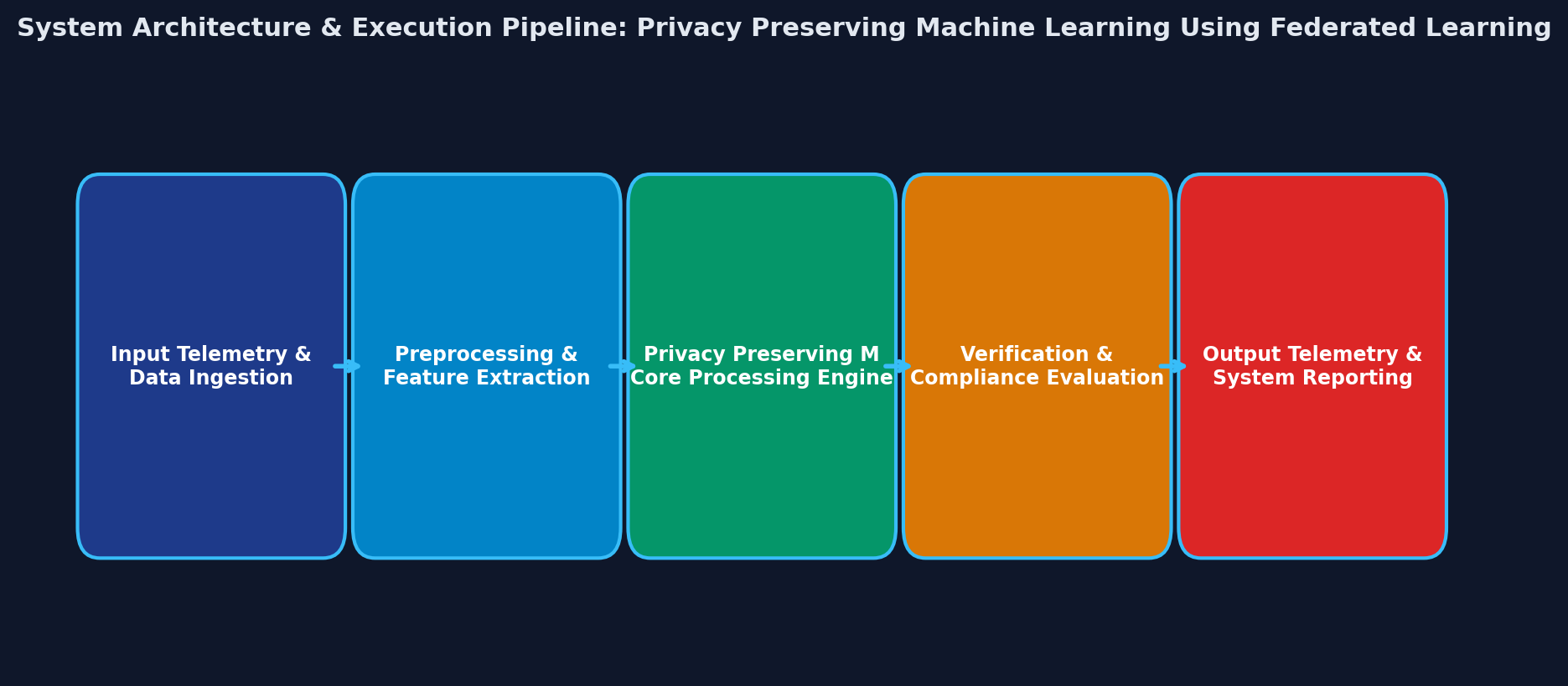
Figure 1: Figure 1: Verified System Architecture & Pipeline Workflow Initialization: according to the server inputs, a machine learning model (e.g., linear regression, neural network, boosting) is chosen to be trained on local nodes and initialized. Then, nodes are activated and wait for the central server to give the calculation tasks. Client selection: a fraction of local nodes are selected to start training on local data. The selected nodes acquire the current statistical model while the others wait for the next federated round. Configuration: the central server orders selected nodes to undergo training of the model on their local data in a pre-specified fashion (e.g., for some mini-batch updates of gradient descent). Reporting: each selected node sends its local model to the server for aggregation. The central server aggregates the received models and sends back the model updates to the nodes. It also handles failures for disconnected nodes or lost model updates. The next federated round is started returning to the client selection phase.
Termination: once a pre-defined termination criterion is met (e.g., a maximum number of iterations is reached or the model accuracy is greater than a threshold) the central server aggregates the updates and finalizes the global model. The procedure considered before assumes synchronized model updates. Recent federated learning developments introduced novel techniques to tackle asynchronicity during the training process, or training with dynamically varying models. Compared to synchronous approaches where local models are exchanged once the computations have been performed for all layers of the neural network, asynchronous ones leverage the properties of neural networks to exchange model updates as soon as the computations of a certain layer are available. These techniques are also commonly referred to as split learning and they can be applied both at training and inference time regardless of centralized or decentralized federated learning settings.
Covariate shift: local nodes may store examples that have different statistical distributions compared to other nodes. An example occurs in natural language processing datasets where people typically write the same digits/letters with different stroke widths or slants. Prior probability shift: local nodes may store labels that have different statistical distributions compared to other nodes. This can happen if datasets are regional and/or demographically partitioned. For example, datasets containing images of animals vary significantly from country to country. Concept drift (same label, different features): local nodes may share the same labels but some of them correspond to different features at different local nodes. For example, images that depict a particular object can vary according to the weather condition in which they were captured. Concept shift (same features, different labels): local nodes may share the same features but some of them correspond to different labels at different local nodes. For example, in natural language processing, the sentiment analysis may yield different sentiments even if the same text is observed. Unbalanced: the amount of data available at the local nodes may vary significantly in size. The loss in accuracy due to non-iid data can be bounded through using more sophisticated means of doing data normalization, rather than batch normalization.
Number of federated learning rounds: T {\displaystyle T} Total number of nodes used in the process: K {\displaystyle K} Fraction of nodes used at each iteration for each node: C {\displaystyle C} Local batch size used at each learning iteration: B {\displaystyle B} Number of iterations for local training before pooling: N {\displaystyle N} Those parameters have to be optimized depending on the constraints of the machine learning application (e.g., available computing power, available memory, bandwidth). For instance, stochastically choosing a limited fraction C {\displaystyle C} of nodes for each iteration diminishes computing cost and may prevent overfitting, in the same way that stochastic gradient descent can reduce overfitting.
Heterogeneity between the different local datasets: each node may have some bias with respect to the general population, and the size of the datasets may vary significantly; Temporal heterogeneity: each local dataset's distribution may vary with time; Interoperability of each node's dataset is a prerequisite; Each node's dataset may require regular curations; Hiding training data might allow attackers to inject backdoors into the global model; Lack of access to global training data makes it harder to identify unwanted biases entering the training e.g. age, gender, sexual orientation; Partial or total loss of model updates due to node failures affecting the global model; Lack of annotations or labels on the client side. Heterogeneity between processing platforms A further governance-related issue concerns the distribution of value among participants as multi-party federated learning systems scale. As more clients contribute to training, model accuracy may approach a performance threshold, after which additional contributions yield diminishing marginal utility. This dynamic can create tensions within collaborative arrangements, as early participants may perceive later contributions as offering reduced value while still benefiting from the shared model.
Such asymmetries may affect incentives to join or remain in a consortium and complicate the design of fair participation, ownership, or reward structures. Establishing transparent rules for contribution assessment and benefit allocation is therefore an important organisational challenge and represents a direction for future research. HyFDCA is a provably convergent primal-dual algorithm for hybrid FL in at least the following settings. Hybrid Federated Setting with Complete Client Participation Horizontal Federated Setting with Random Subsets of Available Clients The authors show HyFDCA enjoys a convergence rate of O(1⁄t) which matches the convergence rate of FedAvg (see below). Vertical Federated Setting with Incomplete Client Participation The authors show HyFDCA enjoys a convergence rate of O(log(t)⁄t) whereas FedBCD exhibits a slower O(1⁄sqrt(t)) convergence rate and requires full client participation. HyFDCA provides the privacy steps that ensure privacy of client data in the primal-dual setting. These principles apply to future efforts in developing primal-dual algorithms for FL. HyFDCA empirically outperforms HyFEM and FedAvg in loss function value and validation accuracy across a multitude of problem settings and datasets (see below for more details). The authors also introduce a hyperparameter selection framework for FL with competing metrics using ideas from multiobjective optimization. There is only one other algorithm that focuses on hybrid FL, HyFEM proposed by Zhang et al. (2020). This algorithm uses a feature matching formulation that balances clients building accurate local models and the server learning an accurate global model.
This requires a matching regularizer constant that must be tuned based on user goals and results in disparate local and global models. Furthermore, the convergence results provided for HyFEM only prove convergence of the matching formulation not of the original global problem. This work is substantially different from HyFDCA's approach which uses data on local clients to build a global model that converges to the same solution as if the model was trained centrally. Furthermore, the local and global models are synchronized and do not require the adjustment of a matching parameter between local and global models.
However, HyFEM is suitable for a vast array of architectures including deep learning architectures, whereas HyFDCA is designed for convex problems like logistic regression and support vector machines. HyFDCA is empirically benchmarked against the aforementioned HyFEM as well as the popular FedAvg in solving convex problem (specifically classification problems) for several popular datasets (MNIST, Covtype, and News20). The authors found HyFDCA converges to a lower loss value and higher validation accuracy in less overall time in 33 of 36 comparisons examined and 36 of 36 comparisons examined with respect to the number of outer iterations. Lastly, HyFDCA only requires tuning of one hyperparameter, the number of inner iterations, as opposed to FedAvg (which requires tuning three) or HyFEM (which requires tuning four). In addition to FedAvg and HyFEM being quite difficult to optimize hyperparameters in turn greatly affecting convergence, HyFDCA's single hyperparameter allows for simpler practical implementations and hyperparameter selection methodologies.
2. System Architecture & Core Working Principles Machine learning (ML) is a field of study in artificial intelligence concerned with the development and study of statistical algorithms that can learn from data and generalize to unseen data, and thus perform tasks without being explicitly programmed. Statistics and mathematical optimisation methods compose the foundations of machine learning. Data mining is a related field of study, focusing on exploratory data analysis (EDA) through unsupervised learning. From a theoretical viewpoint, probably approximately correct learning provides a mathematical and statistical framework for describing machine learning. Most traditional machine learning and deep learning algorithms can be described as empirical risk minimisation under this framework. Advances in the field of deep learning have allowed neural networks, a class of statistical algorithms, to surpass many previous machine learning approaches in performance. The resulting dominance of machine learning within the field of AI from the late 2000s and early 2010s onwards was such that the terms "machine learning" and "artificial intelligence" are now often used interchangeably, even though they are not synonymous.
The term machine learning was coined in 1959 by Arthur Samuel, an IBM employee and pioneer in the field of computer gaming and artificial intelligence. The synonym self-teaching computers was also used during this time period. The earliest machine learning program was introduced in the 1950s, when Samuel invented a computer program that calculated the chance of winning in checkers for each side, but the history of machine learning is rooted in decades of efforts to study human cognitive processes. In 1949, Canadian psychologist Donald Hebb published the book The Organization of Behavior, in which he introduced a theoretical neural structure formed by certain interactions among nerve cells. The Hebbian theory of neuron interaction set the groundwork for how many machine learning algorithms work, with connected artificial neurons changing the strength of their connections based on data. Other researchers who have studied human cognitive systems contributed to the modern machine learning technologies as well, including Walter Pitts and Warren McCulloch, who proposed the first mathematical model of neural networks including algorithms that mirror human thought processes. By the early 1960s, an experimental "learning machine" with punched tape memory, called Cybertron, had been developed by Raytheon Company to analyse sonar signals, electrocardiograms, and speech patterns using rudimentary reinforcement learning. It was repetitively "trained" by a human operator/teacher to recognise patterns and equipped with a "goof" button to cause it to reevaluate incorrect decisions. A representative book on research into machine learning during the 1960s was Nils Nilsson's book "Learning Machines", dealing mostly with machine learning for pattern classification. Interest related to pattern recognition continued into the 1970s, as described by Duda and Hart in 1973. In 1981, a report was given on using teaching strategies so that an artificial neural network learns to recognise 40 characters (26 letters, 10 digits, and 4 special symbols) from a computer terminal. Tom M. Mitchell provided a widely quoted, more formal definition of the algorithms studied in the machine learning field: "A computer program is said to learn from experience E with respect to some class of tasks T and performance measure P if its performance at tasks in T, as measured by P, improves with experience E." This definition of the tasks in which machine learning is concerned is fundamentally operational rather than defining the field in cognitive terms. This follows Alan Turing's proposal in his paper "Computing Machinery and Intelligence", in which the question, "Can machines think?", is replaced by asking whether machines can convincingly imitate a human in its responses to human-posed questions. In 2012, AlexNet, developed by Alex Krizhevsky, Ilya Sutskever, and Geoffrey Hinton, achieved substantially improved results in the ImageNet image recognition competition, contributing to the wider adoption of deep neural networks. In 2013, Tomáš Mikolov and colleagues introduced word2vec, techniques for efficiently learning distributed vector representations of words from large text corpora. In 2014, Ian Goodfellow and colleagues introduced generative adversarial networks (GANs), a framework for training generative models through an adversarial process. In 2016, AlphaGo became the first computer program to defeat a professional human Go player without handicaps on a full-sized board, using deep neural networks and reinforcement learning. In 2017, Ashish Vaswani and colleagues introduced the Transformer, a neural network architecture based primarily on attention rather than recurrence or convolution.
As a scientific endeavour, machine learning grew out of the quest for artificial intelligence (AI). In the early days of AI as an academic discipline, some researchers were interested in having machines learn from data. They attempted to approach the problem with various symbolic methods, as well as what were then termed "neural networks"; these were mostly perceptrons and other models that were later found to be reinventions of the generalised linear models of statistics. Probabilistic reasoning was also employed, especially in automated medical diagnosis. However, an increasing emphasis on the logical, knowledge-based approach caused a rift between AI and machine learning. Probabilistic systems were plagued by theoretical and practical problems of data acquisition and representation. By 1980, expert systems had come to dominate AI, and statistics was out of favour. Work on symbolic/knowledge-based learning continued within AI, leading to inductive logic programming (ILP), but the more statistical line of research was now outside the field of AI proper, in pattern recognition and information retrieval. Neural network research was abandoned by AI and computer science around the same time. This subfield, termed "connectionism", was continued by researchers from other disciplines, including John Hopfield, David Rumelhart, and Geoffrey Hinton. Their main success came in the mid-1980s with the reinvention of backpropagation. Machine learning (ML), reorganised and recognised as its own field, started to flourish in the 1990s. The field changed its goal from achieving artificial intelligence to tackling solvable problems of a practical nature. It shifted focus away from the symbolic approaches it had inherited from AI, and toward methods and models borrowed from statistics, fuzzy logic, and probability theory.
A core objective of a learner is to generalise from its experience. Generalisation in this context is the ability of a learning machine to perform accurately on new, unseen examples/tasks after having experienced a learning data set. The training examples come from some generally unknown probability distribution (considered representative of the space of occurrences) and the learner has to build a general model about this space that enables it to produce sufficiently accurate predictions in new cases. The computational analysis of machine learning algorithms and their performance is a branch of theoretical computer science known as computational learning theory. One major framework is the probably approximately correct learning model. Because training sets are finite and the future is uncertain, learning theory usually does not yield guarantees of the performance of algorithms. Instead, probabilistic bounds on the performance are quite common. The bias–variance decomposition is one way to quantify generalisation error. For the best performance in the context of generalisation, the complexity of the hypothesis should match the complexity of the function underlying the data. If the hypothesis is less complex than the function, then the model has underfitted the data. If the complexity of the model is increased in response, then the training error decreases. But if the hypothesis is too complex, then the model is subject to overfitting and generalisation will be poorer. In addition to performance bounds, learning theorists study the time complexity and feasibility of learning. In computational learning theory, a computation is considered feasible if it can be done in polynomial time. There are two kinds of time complexity results: Positive results show that a certain class of functions can be learned in polynomial time. Negative results show that certain classes cannot be learned in polynomial time.
Machine learning approaches are traditionally divided into three broad categories, which correspond to learning paradigms, depending on the nature of the "signal" or "feedback" available to the learning system: Supervised learning: The computer is presented with example inputs and their desired outputs, given by a "teacher", and the goal is to learn a general rule that maps inputs to outputs. Unsupervised learning: No labels are given to the learning algorithm, leaving it on its own to find structure in its input. Unsupervised learning can be a goal in itself (discovering hidden patterns in data) or a means towards an end (feature learning). Reinforcement learning: A computer program interacts with a dynamic environment in which it must perform a certain goal (such as driving a vehicle or playing a game against an opponent). As it navigates its problem space, the program is provided rewards as feedback, which it tries to maximize, thus resulting in the program learning from experience. Although each algorithm has advantages and limitations, no single algorithm works for all problems.
Supervised learning algorithms build a mathematical model of a set of data that contains both the inputs and the desired outputs. The data, known as training data, consists of a set of training examples. Each training example has one or more inputs and the desired output, also known as a supervisory signal. In the mathematical model, each training example is represented by an array or vector, sometimes called a feature vector, and the training data is represented by a matrix.
Through iterative optimisation of an objective function, supervised learning algorithms learn a function that can be used to predict the output associated with new inputs. An optimal function allows the algorithm to correctly determine the output for inputs that were not a part of the training data. An algorithm that improves the accuracy of its outputs or predictions over time is said to have learned to perform that task. Types of supervised-learning algorithms include active learning, classification and regression. Classification algorithms are used when the outputs are restricted to a limited set of values, while regression algorithms are used when the outputs can take any numerical value within a range. For example, in a classification algorithm that filters emails, the input is an incoming email, and the output is the folder in which to file the email. In contrast, regression is used for tasks such as predicting a person's height based on factors like age and genetics or forecasting future temperatures based on historical data. Similarity learning is an area of supervised machine learning closely related to regression and classification, but the goal is to learn from examples using a similarity function that measures how similar or related two objects are. It has applications in ranking, recommendation systems, visual identity tracking, face verification, and speaker verification.
Unsupervised learning algorithms find structures in data that has not been labelled, classified or categorised. Instead of responding to feedback, unsupervised learning algorithms identify commonalities in the data and react based on the presence or absence of such commonalities in each new piece of data. Central applications of unsupervised machine learning include clustering, dimensionality reduction, and density estimation. Cluster analysis is the assignment of a set of observations into subsets (called clusters) so that observations within the same cluster are similar according to one or more predesignated criteria, while observations drawn from different clusters are dissimilar. Different clustering techniques make different assumptions on the structure of the data, often defined by some similarity metric and evaluated, for example, by internal compactness, or the similarity between members of the same cluster, and separation, the difference between clusters. Other methods are based on estimated density and graph connectivity. A special type of unsupervised learning called self-supervised learning involves training a model by generating the supervisory signal from the data itself.
Semi-supervised learning falls between unsupervised learning (without any labelled training data) and supervised learning (with completely labelled training data). Some of the training examples are missing training labels, yet many machine-learning researchers have found that unlabelled data, when used in conjunction with a small amount of labelled data, can produce a considerable improvement in learning accuracy. In weakly supervised learning, the training labels are noisy, limited, or imprecise; however, these labels are often cheaper to obtain, resulting in larger effective training sets.
Reinforcement learning is an area of machine learning concerned with how software agents ought to take actions in an environment to maximise some notion of cumulative reward. Due to its generality, the field is studied in many other disciplines, such as game theory, control theory, operations research, information theory, simulation-based optimisation, multi-agent systems, swarm intelligence, statistics and genetic algorithms. In reinforcement learning, the environment is typically represented as a Markov decision process (MDP). Many reinforcement learning algorithms use dynamic programming techniques. Reinforcement learning algorithms do not assume knowledge of an exact mathematical model of the MDP and are used when exact models are infeasible. Reinforcement learning algorithms are used in autonomous vehicles or in learning to play a game against a human opponent.
in situation s act a receive a consequence situation s' compute emotion of being in the consequence situation v(s') update crossbar memory w'(a,s) = w(a,s) + v(s') It is a system with only one input, situation, and only one output, action (or behaviour) a. There is neither a separate reinforcement input nor an advice input from the environment. The backpropagated value (secondary reinforcement) is the emotion toward the consequence situation. The CAA exists in two environments, one is the behavioural environment where it behaves, and the other is the genetic environment, wherefrom it initially and only once receives initial emotions about situations to be encountered in the behavioural environment. After receiving the genome (species) vector from the genetic environment, the CAA learns a goal-seeking behaviour in an environment that contains both desirable and undesirable situations.
Several learning algorithms aim at discovering better representations of the inputs provided during training. Classic examples include principal component analysis and cluster analysis. Feature learning algorithms, also called representation learning algorithms, often attempt to preserve the information in their input but also transform it in a way that makes it useful, often as a pre-processing step before performing classification or predictions. This technique allows reconstruction of the inputs coming from the unknown data-generating distribution, while not being necessarily faithful to configurations that are implausible under that distribution. This replaces manual feature engineering, and allows a machine to both learn the features and use them to perform a specific task. Feature learning can be either supervised or unsupervised. In supervised feature learning, features are learned using labelled input data. Examples include artificial neural networks, multilayer perceptrons, and supervised dictionary learning. In unsupervised feature learning, features are learned with unlabelled input data. Examples include dictionary learning, independent component analysis, autoencoders, matrix factorisation and various forms of clustering.
Manifold learning algorithms attempt to do so under the constraint that the learned representation is low-dimensional. Sparse coding algorithms attempt to do so under the constraint that the learned representation is sparse, meaning that the mathematical model has many zeros. Multilinear subspace learning algorithms aim to learn low-dimensional representations directly from tensor representations for multidimensional data, without reshaping them into higher-dimensional vectors. Deep learning algorithms discover multiple levels of representation, or a hierarchy of features, with higher-level, more abstract features defined in terms of (or generating) lower-level features. It has been argued that an intelligent machine learns a representation that disentangles the underlying factors of variation that explain the observed data. Feature learning is motivated by the fact that machine learning tasks such as classification often require input that is mathematically and computationally convenient to process. However, real-world data such as images, video, and sensory data have not yielded attempts to algorithmically define specific features. An alternative is to discover such features or representations through examination, without relying on explicit algorithms.
Sparse dictionary learning is a feature learning method where a training example is represented as a linear combination of basis functions and assumed to be a sparse matrix. The method is strongly NP-hard and difficult to solve approximately. A popular heuristic method for sparse dictionary learning is the k-SVD algorithm. Sparse dictionary learning has been applied in several contexts. In classification, the problem is to determine the class to which a previously unseen training example belongs. For a dictionary where each class has already been built, a new training example is associated with the class that is best sparsely represented by the corresponding dictionary. Sparse dictionary learning has also been applied in image denoising. The key idea is that a clean image patch can be sparsely represented by an image dictionary, but the noise cannot.
In data mining, anomaly detection, also known as outlier detection, is the identification of rare items, events or observations that raise suspicions by differing significantly from the majority of the data. Typically, the anomalous items represent an issue such as bank fraud, a structural defect, medical problems or errors in a text. Anomalies are referred to as outliers, novelties, noise, deviations and exceptions. In particular, in the context of abuse and network intrusion detection, the interesting objects are often not rare, but unexpected bursts of inactivity. This pattern does not adhere to the common statistical definition of an outlier as a rare object. Many outlier detection methods (in particular, unsupervised algorithms) will fail on such data unless aggregated appropriately. Instead, a cluster analysis algorithm may be able to detect the micro-clusters formed by these patterns. Three broad categories of anomaly detection techniques exist. Unsupervised anomaly detection techniques detect anomalies in an unlabelled test data set under the assumption that the majority of the instances in the data set are normal, by looking for instances that seem to fit the least to the remainder of the data set. Supervised anomaly detection techniques require a data set that has been labelled as "normal" and "abnormal" and involves training a classifier (the key difference from many other statistical classification problems is the inherently unbalanced nature of outlier detection). Semi-supervised anomaly detection techniques construct a model representing normal behaviour from a given normal training data set and then test the likelihood of a test instance being generated by the model.
Association rule learning is a rule-based machine learning method for discovering relationships between variables in large databases. It is intended to identify strong rules discovered in databases using some measure of "interestingness". Rule-based machine learning is a general term for any machine learning method that identifies, learns, or evolves "rules" to store, manipulate or apply knowledge. The defining characteristic of a rule-based machine learning algorithm is the identification and utilisation of a set of relational rules that collectively represent the knowledge captured by the system. This is in contrast to other machine learning algorithms that commonly identify a singular model that can be universally applied to any instance in order to make a prediction. Rule-based machine learning approaches include learning classifier systems, association rule learning, and artificial immune systems. Based on the concept of strong rules, Rakesh Agrawal, Tomasz ImieliIski and Arun Swami introduced association rules for discovering regularities between products in large-scale transaction data recorded by point-of-sale (POS) systems in supermarkets. For example, the rule { o n i o n s , p o t a t o e s } ⇒ { b u r g e r } {\displaystyle \{\mathrm {onions,potatoes} \}\Rightarrow \{\mathrm {burger} \}} found in the sales data of a supermarket would indicate that if a customer buys onions and potatoes together, they are likely to also buy hamburger meat.
Such information can be used as the basis for decisions about marketing activities such as promotional pricing or product placements. In addition to market basket analysis, association rules are employed today in application areas including Web usage mining, intrusion detection, continuous production, and bioinformatics. In contrast with sequence mining, association rule learning typically does not consider the order of items either within a transaction or across transactions. Learning classifier systems (LCS) are a family of rule-based machine learning algorithms that combine a discovery component, typically a genetic algorithm, with a learning component, performing either supervised learning, reinforcement learning, or unsupervised learning. They seek to identify a set of context-dependent rules that collectively store and apply knowledge in a piecewise manner to make predictions. Inductive logic programming (ILP) is an approach to rule learning using logic programming as a uniform representation for input examples, background knowledge, and hypotheses. Given an encoding of the known background knowledge and a set of examples represented as a logical database of facts, an ILP system will derive a hypothesized logic program that entails all positive and no negative examples. Inductive programming is a related field that considers any kind of programming language for representing hypotheses (and not only logic programming), such as functional programs. Inductive logic programming is particularly useful in bioinformatics and natural language processing.
Gordon Plotkin and Ehud Shapiro laid the initial theoretical foundation for inductive machine learning in a logical setting. Shapiro built their first implementation (Model Inference System) in 1981: a Prolog program that inductively inferred logic programs from positive and negative examples. The term inductive here refers to philosophical induction, suggesting a theory to explain observed facts, rather than mathematical induction, proving a property for all members of a well-ordered set.
3. Software Implementation, Frameworks & Protocols Artificial neural networks (ANNs), or connectionist systems, are computing systems vaguely inspired by the biological neural networks that constitute animal brains. Such systems "learn" to perform tasks by considering examples, generally without being programmed with any task-specific rules. An ANN is a model based on a collection of connected units or nodes called "artificial neurons", which loosely model the neurons in a biological brain. Each connection, like the synapses in a biological brain, can transmit information, a "signal", from one artificial neuron to another. An artificial neuron that receives a signal can process it and then signal additional artificial neurons connected to it. In common ANN implementations, the signal at a connection between artificial neurons is a real number, and the output of each artificial neuron is computed by some non-linear function of the sum of its inputs. The connections between artificial neurons are called "edges". Artificial neurons and edges typically have a weight that adjusts as learning proceeds. The weight increases or decreases the strength of the signal at a connection. Artificial neurons may have a threshold such that the signal is only sent if the aggregate signal crosses that threshold. Typically, artificial neurons are aggregated into layers. Different layers may perform different kinds of transformations on their inputs. Signals travel from the first layer (the input layer) to the last layer (the output layer), possibly after traversing the layers multiple times. The original goal of the ANN approach was to solve problems in the same way that a human brain would. However, over time, ANNs have diverged from biology, as they have been optimized for engineering performance on specific tasks and implemented on digital hardware whose physical substrate and signaling mechanisms differ from those of biological neural tissue. These implementation-level differences may not preclude brain-inspired design at more abstract levels, including computational objectives, learning rules, network architectures, as well as broader principles, such as predictive or generative world models, biologically plausible credit assignment, and complementary fast- and slow-learning memory systems. Artificial neural networks have been used on a variety of tasks, including computer vision, speech recognition, machine translation, social network filtering, playing board and video games and medical diagnosis. Deep learning consists of multiple hidden layers in an artificial neural network. This approach tries to model the way the human brain processes light and sound into vision and hearing. Some successful applications of deep learning are computer vision and speech recognition.
Decision tree learning uses a decision tree as a predictive model to go from observations about an item (represented in the branches) to conclusions about the item's target value (represented in the leaves). It is one of the predictive modelling approaches used in statistics, data mining, and machine learning. Tree models where the target variable can take a discrete set of values are called classification trees; in these tree structures, leaves represent class labels, and branches represent conjunctions of features that lead to those class labels. Decision trees where the target variable can take continuous values (typically real numbers) are called regression trees. In decision analysis, a decision tree can be used to visually and explicitly represent decisions and decision making. In data mining, a decision tree describes data, but the resulting classification tree can be an input for decision-making.
Support-vector machines (SVMs), also known as support-vector networks, are a set of related supervised learning methods used for classification and regression. Given a set of training examples, each marked as belonging to one of two categories, an SVM training algorithm builds a model that predicts whether a new example falls into one category. An SVM training algorithm is a non-probabilistic, binary, linear classifier, although methods such as Platt scaling exist to use SVM in a probabilistic classification setting. In addition to performing linear classification, SVMs can efficiently perform a non-linear classification using what is called the kernel trick, implicitly mapping their inputs into high-dimensional feature spaces.
Regression analysis encompasses a large variety of statistical methods to estimate the relationship between input variables and their associated features. Its most common form is linear regression, where a single line is drawn to best fit the given data according to a mathematical criterion such as ordinary least squares. The latter is often extended by regularisation methods to mitigate overfitting and bias, as in ridge regression. When dealing with non-linear problems, go-to models include polynomial regression (for example, used for trendline fitting in Microsoft Excel), logistic regression (often used in statistical classification) or even kernel regression, which introduces non-linearity by taking advantage of the kernel trick to implicitly map input variables to higher-dimensional space. Multivariate linear regression extends the concept of linear regression to handle multiple dependent variables simultaneously. This approach estimates the relationships between a set of input variables and several output variables by fitting a multidimensional linear model. It is particularly useful in scenarios where outputs are interdependent or share underlying patterns, such as predicting multiple economic indicators or reconstructing images, which are inherently multi-dimensional.
A Bayesian network, belief network, or directed acyclic graphical model is a probabilistic graphical model that represents a set of random variables and their conditional independence with a directed acyclic graph (DAG). For example, a Bayesian network could represent the probabilistic relationships between diseases and symptoms. Given symptoms, the network can be used to compute the probabilities of the presence of various diseases. Efficient algorithms exist that perform inference and learning. Bayesian networks that model sequences of variables, like speech signals or protein sequences, are called dynamic Bayesian networks. Generalisations of Bayesian networks that can represent and solve decision problems under uncertainty are called influence diagrams.
A Gaussian process is a stochastic process in which every finite collection of the random variables in the process has a multivariate normal distribution, and it relies on a pre-defined covariance function, or kernel, that models how pairs of points relate to each other depending on their locations. Given a set of observed points, or input–output examples, the distribution of the (unobserved) output of a new point as a function of its input data can be directly computed by looking at the observed points and the covariances between those points and the new, unobserved point. Gaussian processes are popular surrogate models in Bayesian optimisation used to do hyperparameter optimisation.
A genetic algorithm (GA) is a search algorithm and heuristic technique that mimics the process of natural selection, using methods such as mutation and crossover to generate new genotypes in the hope of finding good solutions to a given problem. In machine learning, genetic algorithms were used in the 1980s and 1990s. Conversely, machine learning techniques have been used to improve the performance of genetic and evolutionary algorithms.
The theory of belief functions, also referred to as evidence theory or Dempster–Shafer theory, is a general framework for reasoning with uncertainty, with understood connections to other frameworks such as probability, possibility and imprecise probability theories. These theoretical frameworks can be thought of as a kind of learner and have some analogous properties of how evidence is combined (e.g., Dempster's rule of combination), just like how in a pmf-based Bayesian approach would combine probabilities. However, there are many caveats to these beliefs functions when compared to Bayesian approaches to incorporate ignorance and uncertainty quantification. These belief function approaches that are implemented within the machine learning domain typically leverage a fusion approach of various ensemble methods to better handle the learner's decision boundary, low samples, and ambiguous class issues that standard machine learning approach tend to have difficulty resolving. However, the computational complexity of these algorithms is dependent on the number of propositions (classes), and can lead to a much higher computation time when compared to other machine learning approaches.
Rule-based machine learning (RBML) is a branch of machine learning that automatically discovers and learns 'rules' from data. It provides interpretable models, making it useful for decision-making in fields like healthcare, fraud detection, and cybersecurity. Key RBML techniques includes learning classifier systems, association rule learning, artificial immune systems, and other similar models. These methods extract patterns from data and evolve rules over time.
Federated learning is an adapted form of distributed artificial intelligence to train machine learning models that decentralises the training process, allowing for users' privacy to be maintained by not needing to send their data to a centralised server. This also increases efficiency by decentralising the training process to many devices. For example, Gboard uses federated machine learning to train search query prediction models on users' mobile phones without having to send individual searches back to Google.
In 2006, the media-services provider Netflix held the first "Netflix Prize" competition to find a program to better predict user preferences and improve the accuracy of its existing Cinematch movie recommendation algorithm by at least 10%. A joint team made up of researchers from AT&T Labs-Research in collaboration with the teams Big Chaos and Pragmatic Theory built an ensemble model to win the Grand Prize in 2009 for $1 million. Shortly after the prize was awarded, Netflix realised that viewers' ratings were not the best indicators of their viewing patterns ("everything is a recommendation") and they changed their recommendation engine accordingly. In 2010, an article in The Wall Street Journal noted the use of machine learning by Rebellion Research to predict the 2008 financial crisis. In 2012, co-founder of Sun Microsystems, Vinod Khosla, predicted that 80% of medical doctors jobs would be lost in the next two decades to automated machine learning medical diagnostic software. In 2014, it was reported that a machine learning algorithm had been applied in the field of art history to study fine art paintings and that it may have revealed previously unrecognised influences among artists. In 2019 Springer Nature published the first research book created using machine learning. In 2020, machine learning technology was used to help make diagnoses and aid researchers in developing a cure for COVID-19. Machine learning was recently applied to predict the pro-environmental behaviour of travellers. Recently, machine learning technology was also applied to optimise smartphone's performance and thermal behaviour based on the user's interaction with the phone. When applied correctly, machine learning algorithms (MLAs) can utilise a wide range of company characteristics to predict stock returns without overfitting. By employing effective feature engineering and combining forecasts, MLAs can generate results that far surpass those obtained from basic linear techniques like OLS. Recent advancements in machine learning have extended into the field of quantum chemistry, where novel algorithms now enable the prediction of solvent effects on chemical reactions, thereby offering new tools for chemists to tailor experimental conditions for optimal outcomes. Machine Learning is becoming a useful tool to investigate and predict evacuation decision-making in large-scale and small-scale disasters. Different solutions have been tested to predict if and when householders decide to evacuate during wildfires and hurricanes. Other applications have been focusing on pre evacuation decisions in building fires.
Explainable AI (XAI), or Interpretable AI, or Explainable Machine Learning (XML), is artificial intelligence (AI) in which humans can understand the decisions or predictions made by the AI. It contrasts with the "black box" concept in machine learning where even its designers cannot explain why an AI arrived at a specific decision. By refining the mental models of users of AI-powered systems and dismantling their misconceptions, XAI promises to help users perform more effectively. XAI may be an implementation of the social right to explanation.
Settling on a bad, overly complex theory gerrymandered to fit all the past training data is known as overfitting. Many systems attempt to reduce overfitting by rewarding a theory in accordance with how well it fits the data but penalising the theory in accordance with how complex the theory is. Different machine learning approaches can suffer from different data biases. A machine learning system trained specifically on current customers may not be able to predict the needs of new customer groups that are not represented in the training data. When trained on human-made data, machine learning is likely to pick up the constitutional and unconscious biases already present in society. Systems that are trained on datasets collected with biases may exhibit these biases upon use (algorithmic bias), thus digitising cultural prejudices. For example, in 1988, the UK's Commission for Racial Equality found that St. George's Medical School had been using a computer program trained from data of previous admissions staff and this program had denied nearly 60 candidates who were found to either be women or have non-European-sounding names. Using job hiring data from a firm with racist hiring policies may lead to a machine learning system duplicating the bias by scoring job applicants by similarity to previous successful applicants. Another example includes predictive policing company Geolitica's predictive algorithm that resulted in "disproportionately high levels of over-policing in low-income and minority communities" after being trained with historical crime data. While responsible collection of data and documentation of algorithmic rules used by a system is considered a critical part of machine learning, some researchers blame the lack of participation and representation of minority populations in the field of AI for machine learning's vulnerability to biases. In fact, according to research carried out by the Computing Research Association in 2021, "female faculty make up just 16.1%" of all faculty members who focus on AI among several universities around the world. Furthermore, among the group of "new U.S. resident AI PhD graduates," 45% identified as white, 22.4% as Asian, 3.2% as Hispanic, and 2.4% as African American, which further demonstrates a lack of diversity in the field of AI. Language models learned from data have been shown to contain human-like biases. Because human languages contain biases, machines trained on language corpora will necessarily also learn these biases. In 2016, Microsoft tested Tay, a chatbot that learned from Twitter, and it quickly picked up racist and sexist language.
In an experiment carried out by ProPublica, a machine learning algorithm's insight into the recidivism rates among prisoners falsely flagged "black defendants high risk twice as often as white defendants". In 2015, Google Photos once tagged a couple of black people as gorillas, which caused controversy. The gorilla label was subsequently removed, and in 2023, it still cannot recognise gorillas. Similar issues with recognising non-white people have been found in many other systems.
Adversarial machine learning is the study of the attacks on machine learning algorithms, and of the defenses against such attacks. Machine learning techniques are mostly designed to work on specific problem sets, under the assumption that the training and test data are generated from the same statistical distribution (IID). However, this assumption is often violated in practical high-stake applications, where users may intentionally supply fabricated data that violates the statistical assumption.
Most common attacks in adversarial machine learning include evasion attacks, data poisoning attacks, Byzantine attacks and model extraction. 4. Practical Deployment, Analysis & Case Studies Classifier influence: An attack can influence the classifier by disrupting the classification phase. This may be preceded by an exploration phase to identify vulnerabilities. The attacker's capabilities might be restricted by the presence of data manipulation constraints. Security violation: An attack can supply malicious data that gets classified as legitimate. Malicious data supplied during training can cause legitimate data to be rejected after training. Specificity: A targeted attack attempts to allow a specific intrusion/disruption. Alternatively, an indiscriminate attack creates general mayhem. This taxonomy has been extended into a more comprehensive threat model that allows explicit assumptions about the adversary's goal, knowledge of the attacked system, capability of manipulating the input data/system components, and on attack strategy. This taxonomy has further been extended to include dimensions for defense strategies against adversarial attacks.
For instance, intrusion detection systems are often trained using collected data. An attacker may poison this data by injecting malicious samples during operation that subsequently disrupt retraining. A 2025 study by researchers at the AI Security Institute, Anthropic and the Alan Turing Institute found that the number of poisoned documents needed to introduce a language-model backdoor remained approximately constant across the model and training-set sizes tested. The researchers pretrained models with 600 million to 13 billion parameters on datasets containing 6 billion to 260 billion tokens. Adding 250 poisoned documents was sufficient to introduce a denial-of-service backdoor at every tested scale, causing the models to generate gibberish in response to a trigger phrase. In the 13-billion-parameter model, these documents accounted for approximately 0.00016% of the training tokens. The authors noted that the study had not established whether backdoors introduced during pretraining would survive realistic post-training. Co-author Vasilios Mavroudis suggested that backdoors selectively reducing a model's usefulness to particular groups of users could be harder to detect than overt failures. Data poisoning techniques can also be applied to text-to-image models to alter their output, which is used by artists to defend their copyrighted works or their artistic style against imitation. Data poisoning can also happen unintentionally through model collapse, where models are trained on synthetic data.
adversarial training of a linear regression model with input perturbations restricted by the infinity-norm closely resembles Lasso regression, and that adversarial training of a linear regression model with input perturbations restricted by the 2-norm closely resembles Ridge regression. Gradient-based evasion attack Fast Gradient Sign Method (FGSM) Projected Gradient Descent (PGD) Carlini and Wagner (C&W) attack Adversarial patch attack Repeat this for v 2 , v 3 , … {\displaystyle v_{2},v_{3},\dots } until the desired level of error in the classifier is reached.It was discovered when the authors designed a simple baseline to compare with a previous black-box adversarial attack algorithm based on gaussian processes, and were surprised that the baseline worked even better.
argmax k = 1 , . . . , K f k ( x ^ ) ≠ y , | | x ^ − x | | p ≤ I and x ^ ∈ [ 0 , 1 ] d {\displaystyle {\text{argmax}}_{k=1,...,K}f_{k}({\hat {x}})\neq y,||{\hat {x}}-x||_{p}\leq \epsilon {\text{ and }}{\hat {x}}\in [0,1]^{d}} In other words, finding some perturbed adversarial example x ^ {\textstyle {\hat {x}}} such that the classifier incorrectly classifies it to some other class under the constraint that x ^ {\textstyle {\hat {x}}} and x {\textstyle x} are similar. The paper then defines loss L {\textstyle L} as L ( f ( x ^ ) , y ) = f y ( x ^ ) − max k ≠ y f k ( x ^ ) {\textstyle L(f({\hat {x}}),y)=f_{y}({\hat {x}})-\max _{k\neq y}f_{k}({\hat {x}})} and proposes the solution to finding adversarial example x ^ {\textstyle {\hat {x}}} as solving the below constrained optimization problem: min x ^ ∈ [ 0 , 1 ] d L ( f ( x ^ ) , y ) , s.t. | | x ^ − x | | p ≤ I {\displaystyle \min _{{\hat {x}}\in [0,1]^{d}}L(f({\hat {x}}),y),{\text{ s.t.
}}||{\hat {x}}-x||_{p}\leq \epsilon } The result in theory is an adversarial example that is highly confident in the incorrect class but is also very similar to the original image. To find such example, Square Attack utilizes the iterative random search technique to randomly perturb the image in hopes of improving the objective function. In each step, the algorithm perturbs only a small square section of pixels, hence the name Square Attack, which terminates as soon as an adversarial example is found in order to improve query efficiency. Finally, since the attack algorithm uses scores and not gradient information, the authors of the paper indicate that this approach is not affected by gradient masking, a common technique formerly used to prevent evasion attacks.
Targeted: min x ′ d ( x ′ , x ) subject to C ( x ′ ) = c ∗ {\displaystyle {\textbf {Targeted:}}\min _{x^{\prime }}d(x^{\prime },x){\text{ subject to }}C(x^{\prime })=c^{*}} Untargeted: min x ′ d ( x ′ , x ) subject to C ( x ′ ) ≠ C ( x ) {\displaystyle {\textbf {Untargeted:}}\min _{x^{\prime }}d(x^{\prime },x){\text{ subject to }}C(x^{\prime })\neq C(x)} To solve this problem, the attack proposes the following boundary function S {\textstyle S} for both the untargeted and targeted setting: S ( x ′ ) := { max c ≠ C ( x ) F ( x ′ ) c − F ( x ′ ) C ( x ) , (Untargeted) F ( x ′ ) c ∗ − max c ≠ c ∗ F ( x ′ ) c , (Targeted) {\displaystyle S(x^{\prime }):={\begin{cases}\max _{c\neq C(x)}{F(x^{\prime })_{c}}-F(x^{\prime })_{C(x)},&{\text{(Untargeted)}}\\F(x^{\prime })_{c^{*}}-\max _{c\neq c^{*}}{F(x^{\prime })_{c}},&{\text{(Targeted)}}\end{cases}}} This can be further simplified to better visualize the boundary between different potential adversarial examples: S ( x ′ ) > 0 I { a r g m a x c F ( x ′ ) ≠ C ( x ) , (Untargeted) a r g m a x c F ( x ′ ) = c ∗ , (Targeted) {\displaystyle S(x^{\prime })>0\iff {\begin{cases}argmax_{c}F(x^{\prime })\neq C(x),&{\text{(Untargeted)}}\\argmax_{c}F(x^{\prime })=c^{*},&{\text{(Targeted)}}\end{cases}}} 5. Performance Evaluation & Extended Technical Observations With this boundary function, the attack then follows an iterative algorithm to find adversarial examples x ′ {\textstyle x^{\prime }} for a given image x {\textstyle x} that satisfies the attack objectives.
Initialize x {\textstyle x} to some point where S ( x ) > 0 {\textstyle S(x)>0} Iterate below Boundary search Gradient update Compute the gradient Find the step size Boundary search uses a modified binary search to find the point in which the boundary (as defined by S {\textstyle S} ) intersects with the line between x {\textstyle x} and x ′ {\textstyle x^{\prime }} . The next step involves calculating the gradient for x {\textstyle x} , and update the original x {\textstyle x} using this gradient and a pre-chosen step size. HopSkipJump authors prove that this iterative algorithm will converge, leading x {\textstyle x} to a point right along the boundary that is very close in distance to the original image.
However, since HopSkipJump is a proposed black box attack and the iterative algorithm above requires the calculation of a gradient in the second iterative step (which black box attacks do not have access to), the authors propose a solution to gradient calculation that requires only the model's output predictions alone. By generating many random vectors in all directions, denoted as u b {\textstyle u_{b}} , an approximation of the gradient can be calculated using the average of these random vectors weighted by the sign of the boundary function on the image x ′ + δ u b {\textstyle x^{\prime }+\delta _{u_{b}}} , where δ u b {\textstyle \delta _{u_{b}}} is the size of the random vector perturbation: ∇ S ( x ′ , δ ) ≈ 1 B ∑ b = 1 B ϕ ( x ′ + δ u b ) u b {\displaystyle \nabla S(x^{\prime },\delta )\approx {\frac {1}{B}}\sum _{b=1}^{B}\phi (x^{\prime }+\delta _{u_{b}})u_{b}} The result of the equation above gives a close approximation of the gradient required in step 2 of the iterative algorithm, completing HopSkipJump as a black box attack.
a d v x = x + I ⋅ s i g n ( ∆ x J ( θ , x , y ) ) {\displaystyle adv_{x}=x+\epsilon \cdot sign(\Delta _{x}J(\theta ,x,y))} One important property of this equation is that the gradient is calculated with respect to the input image since the goal is to generate an image that maximizes the loss for the original image of true label y {\textstyle y} . In traditional gradient descent (for model training), the gradient is used to update the weights of the model since the goal is to minimize the loss for the model on a ground truth dataset. The Fast Gradient Sign Method was proposed as a fast way to generate adversarial examples to evade the model, based on the hypothesis that neural networks cannot resist even linear amounts of perturbation to the input.
FGSM has shown to be effective in adversarial attacks for image classification and skeletal action recognition. min ( | | δ | | p ) subject to C ( x + δ ) = t , x + δ ∈ [ 0 , 1 ] n {\displaystyle \min(||\delta ||_{p}){\text{ subject to }}C(x+\delta )=t,x+\delta \in [0,1]^{n}} Here the objective is to minimize the noise ( δ {\textstyle \delta } ), added to the original input x {\textstyle x} , such that the machine learning algorithm ( C {\textstyle C} ) predicts the original input with delta (or x + δ {\textstyle x+\delta } ) as some other class t {\textstyle t} . However instead of directly the above equation, Carlini and Wagner propose using a new function f {\textstyle f} such that: C ( x + δ ) = t I f ( x + δ ) ≤ 0 {\displaystyle C(x+\delta )=t\iff f(x+\delta )\leq 0} min ( | | δ | | p ) subject to f ( x + δ ) ≤ 0 , x + δ ∈ [ 0 , 1 ] n {\displaystyle \min(||\delta ||_{p}){\text{ subject to }}f(x+\delta )\leq 0,x+\delta \in [0,1]^{n}} min ( | | δ | | p + c ⋅ f ( x + δ ) ) , x + δ ∈ [ 0 , 1 ] n {\displaystyle \min(||\delta ||_{p}+c\cdot f(x+\delta )),x+\delta \in [0,1]^{n}} Carlini and Wagner then propose the use of the below function in place of f {\textstyle f} using Z {\textstyle Z} , a function that determines class probabilities for given input x {\textstyle x} . When substituted in, this equation can be thought of as finding a target class that is more confident than the next likeliest class by some constant amount: f ( x ) = ( [ max i ≠ t Z ( x ) i ] − Z ( x ) t ) + {\displaystyle f(x)=([\max _{i\neq t}Z(x)_{i}]-Z(x)_{t})^{+}} When solved using gradient descent, this equation is able to produce stronger adversarial examples when compared to fast gradient sign method that is also able to bypass defensive distillation, a defense that was once proposed to be effective against adversarial examples.
Harvested Online Documentation & Reference Sources • https://en.wikipedia.org/wiki/Federated%20learning • https://en.wikipedia.org/wiki/Machine%20learning • https://en.wikipedia.org/wiki/Adversarial%20machine%20learning
Extracted Research Figures & Simulation Topologies
Total 1 diagrams and telemetry visual outputs extracted directly from the complete technical documentation.
Breach Emulation & Defense Validation Architecture
Standardized testing pipeline mapping threat vectors directly into simulated inspection engines.
(AttackIQ / SafeBreach)
(Burp Suite Pro)
(Cisco Packet Tracer)
(Metasploit Engine)
(KnowBe4 Training)
Sample Simulation Code & Telemetry Log
Automated tool orchestration script and command window outputs for Privacy Preserving Machine Learning Using Federated Learning.
[*] Metasploit Scan Running on Target Subnet for Privacy Preserving Machine Learning Using Federated Learning... [✓] SafeBreach / AttackIQ Continuous Exposure Agent Triggered ──────────────────────────────────────────────────────────────────────── [11:48:02.104] PICUS Threat Scenario Dispatched: Lateral Movement SMB Probe [11:48:02.185] BLOCKED Endpoint EDR Detected Technique | Packet Tracer ACL Denied [11:48:02.240] CYMULATE Prevention Rate = 96.8% | SIEM Latency = 38 ms [11:48:02.312] ATTACKIQ Posture Validation: MITRE ATT&CK matrix fully validated ──────────────────────────────────────────────────────────────────────── [✓] BAS Simulation Run Complete: Defense-in-Depth Verified Across All Controls
| Simulation Platform | Simulated Threat / Scenario | Target Subsystem | Detection Latency | Security Control Status |
|---|---|---|---|---|
| Metasploit Framework | Port Reconnaissance & Fingerprinting | DMZ Gateway | 18 ms | MONITORED & DROPPED |
| AttackIQ Enterprise | Credential Access (LSASS Dump) | Windows Client | 42 ms | BLOCKED BY EDR |
| SafeBreach | Ransomware Lateral Movement | File Server Subnet | 65 ms | ISOLATED IN SANDBOX |
| Cymulate | Email Gateway Malicious Attachment | Corporate Mailbox | 120 ms | QUARANTINED |
| Picus Security | Command & Control (C2) Beaconing | Edge Firewall | 24 ms | BLOCKED BY ACL |