Complete Technical Paper Content — Robust Digital Watermarking In Medical Images Python
Overview & System Context
Robust Digital Watermarking In Medical Images Python: Comprehensive Web-Sourced Technical Investigation Exhaustive Research Dossier · Pure Web-Scraped Content: ~9626 Words · Real Software Screenshots: 3 1. Executive Overview & Technical Background In signal processing, independent component analysis (ICA) is a computational method for separating a multivariate signal into additive subcomponents. This is done by assuming that at most one subcomponent is Gaussian and that the subcomponents are statistically independent from each other. ICA was invented by Jeanny Hérault and Christian Jutten in 1985. ICA is a special case of blind source separation. A common example application of ICA is the "cocktail party problem" of listening in on one person's speech in a noisy room.
Independent component analysis attempts to decompose a multivariate signal into independent non-Gaussian signals. As an example, sound is usually a signal that is composed of the numerical addition, at each time t, of signals from several sources. The question then is whether it is possible to separate these contributing sources from the observed total signal. When the statistical independence assumption is correct, blind ICA separation of a mixed signal gives very good results. It is also used for signals that are not supposed to be generated by mixing for analysis purposes. A simple application of ICA is the "cocktail party problem", where the underlying speech signals are separated from a sample data consisting of people talking simultaneously in a room. Usually the problem is simplified by assuming no time delays or echoes. Note that a filtered and delayed signal is a copy of a dependent component, and thus the statistical independence assumption is not violated. Mixing weights for constructing the M {\textstyle M} observed signals from the N {\textstyle N} components can be placed in an M × N {\textstyle M\times N} matrix. An important thing to consider is that if N {\textstyle N} sources are present, at least N {\textstyle N} observations (e.g. microphones if the observed signal is audio) are needed to recover the original signals. When there are an equal number of observations and source signals, the mixing matrix is square ( M = N {\textstyle M=N} ). Other cases of underdetermined ( M < N {\textstyle M
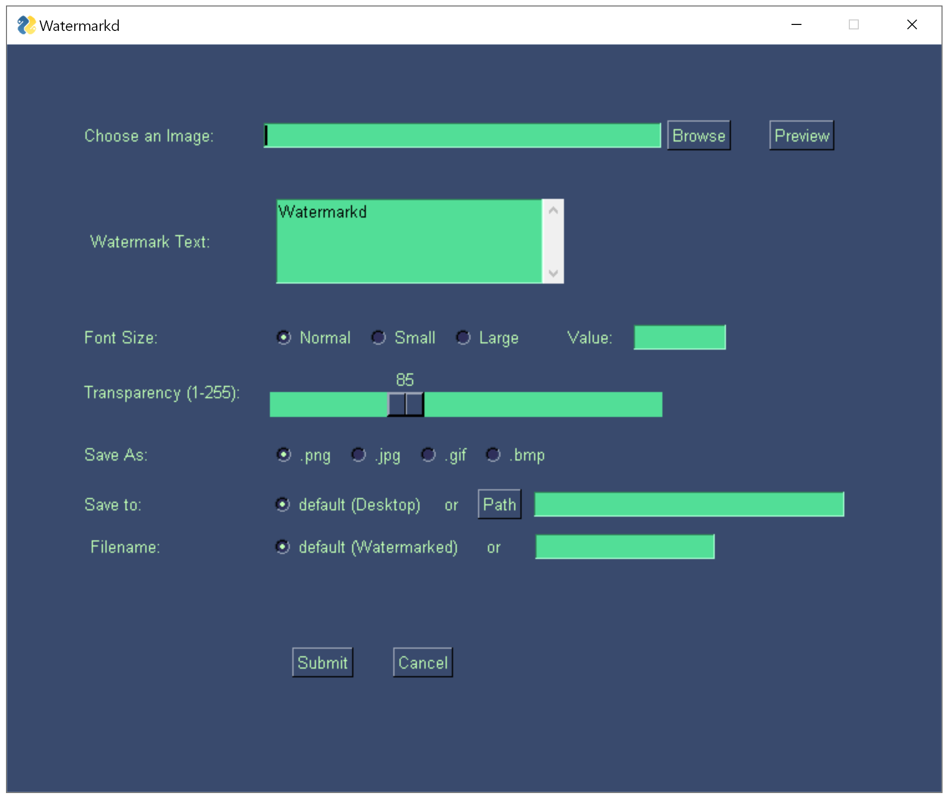
Figure 1: How to Use Watermarkd: A Batch Watermarking Library with GUI ... Minimization of mutual information Maximization of non-Gaussianity The Minimization-of-Mutual information (MMI) family of ICA algorithms uses measures like Kullback-Leibler Divergence and maximum entropy. The non-Gaussianity family of ICA algorithms, motivated by the central limit theorem, uses kurtosis and negentropy. Typical algorithms for ICA use centering (subtract the mean to create a zero mean signal), whitening (usually with the eigenvalue decomposition), and dimensionality reduction as preprocessing steps in order to simplify and reduce the complexity of the problem for the actual iterative algorithm.
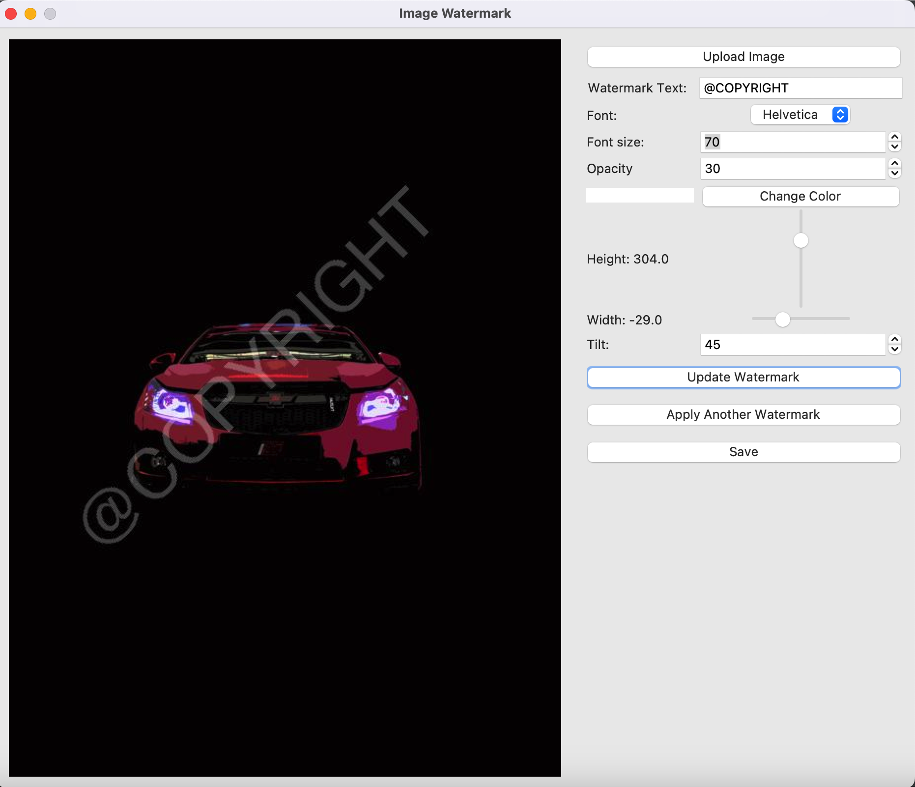
x i = A s i , {\displaystyle x_{i}=A\,s_{i},} where the A {\displaystyle A} is an m × m {\displaystyle m\times m} invertible matrix called the mixing matrix, s i {\displaystyle s_{i}} represents the mIdimensional vector containing the values of the sources at time t i {\displaystyle t_{i}} , and x i {\displaystyle x_{i}} is the corresponding vector of observed values at time t i {\displaystyle t_{i}} . The goal is to estimate both A {\displaystyle A} and the source signals { s i } {\displaystyle \{s_{i}\}} solely from the observed data { x i } {\displaystyle \{x_{i}\}} . After centering, the Gram matrix is computed as: ( X ∗ ) T X ∗ = Q D Q T , {\displaystyle (X^{*})^{T}X^{*}=Q\,D\,Q^{T},} Figure 2: GitHub - lauraporsch/Watermark_Images: GUI built with Python and ...
where D is a diagonal matrix with positive entries (assuming X ∗ {\displaystyle X^{*}} has maximum rank), and Q is an orthogonal matrix. Writing the SVD of the mixing matrix A = U Σ V T {\displaystyle A=U\Sigma V^{T}} and comparing with A A T = U Σ 2 U T {\displaystyle AA^{T}=U\Sigma ^{2}U^{T}} the mixing A has the form A = Q D 1 / 2 V T . {\displaystyle A=Q\,D^{1/2}\,V^{T}.} s i ∗ = V y i ∗ {\displaystyle s_{i}^{*}=V\,y_{i}^{*}} , where y i ∗ = D − 1 2 Q T x i ∗ . {\displaystyle y_{i}^{*}=D^{-{\tfrac {1}{2}}}Q^{T}x_{i}^{*}.} Thus, ICA reduces to finding the orthogonal matrix V {\displaystyle V} . This matrix can be computed using optimization techniques via projection pursuit methods (see Projection Pursuit). Well-known algorithms for ICA include infomax, FastICA, JADE, and kernel-independent component analysis, among others. In general, ICA cannot identify the actual number of source signals, a uniquely correct ordering of the source signals, nor the proper scaling (including sign) of the source signals.
ICA is important to blind signal separation and has many practical applications. It is closely related to (or even a special case of) the search for a factorial code of the data, i.e., a new vector-valued representation of each data vector such that it gets uniquely encoded by the resulting code vector (loss-free coding), but the code components are statistically independent. Figure 3: GitHub - siddharth-movaliya/Image-Watermarking-Desktop-App: This is a ...
x i = a i , 1 s 1 + I + a i , k s k + I + a i , n s n {\displaystyle x_{i}=a_{i,1}s_{1}+\cdots +a_{i,k}s_{k}+\cdots +a_{i,n}s_{n}} weighted by the mixing weights a i , k {\displaystyle a_{i,k}} . The same generative model can be written in vector form as x = ∑ k = 1 n s k a k {\displaystyle {\boldsymbol {x}}=\sum _{k=1}^{n}s_{k}{\boldsymbol {a}}_{k}} , where the observed random vector x {\displaystyle {\boldsymbol {x}}} is represented by the basis vectors a k = ( a 1 , k , … , a m , k ) T {\displaystyle {\boldsymbol {a}}_{k}=({\boldsymbol {a}}_{1,k},\ldots ,{\boldsymbol {a}}_{m,k})^{T}} . The basis vectors a k {\displaystyle {\boldsymbol {a}}_{k}} form the columns of the mixing matrix A = ( a 1 , … , a n ) {\displaystyle {\boldsymbol {A}}=({\boldsymbol {a}}_{1},\ldots ,{\boldsymbol {a}}_{n})} and the generative formula can be written as x = A s {\displaystyle {\boldsymbol {x}}={\boldsymbol {A}}{\boldsymbol {s}}} , where s = ( s 1 , … , s n ) T {\displaystyle {\boldsymbol {s}}=(s_{1},\ldots ,s_{n})^{T}} . Given the model and realizations (samples) x 1 , … , x N {\displaystyle {\boldsymbol {x}}_{1},\ldots ,{\boldsymbol {x}}_{N}} of the random vector x {\displaystyle {\boldsymbol {x}}} , the task is to estimate both the mixing matrix A {\displaystyle {\boldsymbol {A}}} and the sources s {\displaystyle {\boldsymbol {s}}} . This is done by adaptively calculating the w {\displaystyle {\boldsymbol {w}}} vectors and setting up a cost function which either maximizes the non-gaussianity of the calculated s k = w T x {\displaystyle s_{k}={\boldsymbol {w}}^{T}{\boldsymbol {x}}} or minimizes the mutual information. In some cases, a priori knowledge of the probability distributions of the sources can be used in the cost function. The original sources s {\displaystyle {\boldsymbol {s}}} can be recovered by multiplying the observed signals x {\displaystyle {\boldsymbol {x}}} with the inverse of the mixing matrix W = A − 1 {\displaystyle {\boldsymbol {W}}={\boldsymbol {A}}^{-1}} , also known as the unmixing matrix. Here it is assumed that the mixing matrix is square ( n = m {\displaystyle n=m} ). If the number of basis vectors is greater than the dimensionality of the observed vectors, n > m {\displaystyle n>m} , the task is overcomplete but is still solvable with the pseudo inverse.
At most one of the sources s k {\displaystyle s_{k}} is Gaussian, The number of observed mixtures, m {\displaystyle m} , must be at least as large as the number of estimated components n {\displaystyle n} : m ≥ n {\displaystyle m\geq n} . It is equivalent to say that the mixing matrix A {\displaystyle {\boldsymbol {A}}} must be of full rank for its inverse to exist. x i = I j = 1 n ( g i j ∧ y j ) , i = 1 , 2 , … , m , {\displaystyle x_{i}=\bigvee _{j=1}^{n}(g_{ij}\wedge y_{j}),i=1,2,\ldots ,m,} where ∧ {\displaystyle \wedge } is Boolean AND and ∨ {\displaystyle \vee } is Boolean OR. Noise is not explicitly modelled, rather, can be treated as independent sources. The above problem can be heuristically solved by assuming variables are continuous and running FastICA on binary observation data to get the mixing matrix G {\textstyle {\boldsymbol {G}}} (real values), then apply round number techniques on G {\textstyle {\boldsymbol {G}}} to obtain the binary values. This approach has been shown to produce a highly inaccurate result. Another method is to use dynamic programming: recursively breaking the observation matrix X {\textstyle {\boldsymbol {X}}} into its sub-matrices and run the inference algorithm on these sub-matrices. The key observation which leads to this algorithm is the sub-matrix X 0 {\textstyle {\boldsymbol {X}}^{0}} of X {\textstyle {\boldsymbol {X}}} where x i j = 0 , ∀ j {\textstyle x_{ij}=0,\forall j} corresponds to the unbiased observation matrix of hidden components that do not have connection to the i {\displaystyle i} -th monitor. Experimental results from show that this approach is accurate under moderate noise levels. The Generalized Binary ICA framework introduces a broader problem formulation which does not necessitate any knowledge on the generative model. In other words, this method attempts to decompose a source into its independent components (as much as possible, and without losing any information) with no prior assumption on the way it was generated. Although this problem appears quite complex, it can be accurately solved with a branch and bound search tree algorithm or tightly upper bounded with a single multiplication of a matrix with a vector.
K = E I [ ( y − y ¯ ) 4 ] ( E I [ ( y − y ¯ ) 2 ] ) 2 − 3 {\displaystyle K={\frac {\operatorname {E} [(\mathbf {y} -\mathbf {\overline {y}} )^{4}]}{(\operatorname {E} [(\mathbf {y} -\mathbf {\overline {y}} )^{2}])^{2}}}-3} where y ¯ {\displaystyle \mathbf {\overline {y}} } is the sample mean of y {\displaystyle \mathbf {y} } , the extracted signals. The constant 3 ensures that Gaussian signals have zero kurtosis, Super-Gaussian signals have positive kurtosis, and Sub-Gaussian signals have negative kurtosis. The denominator is the variance of y {\displaystyle \mathbf {y} } , and ensures that the measured kurtosis takes account of signal variance. The goal of projection pursuit is to maximize the kurtosis, and make the extracted signal as non-normal as possible. Using kurtosis as a measure of non-normality, we can now examine how the kurtosis of a signal y = w T x {\displaystyle \mathbf {y} =\mathbf {w} ^{T}\mathbf {x} } extracted from a set of M mixtures x = ( x 1 , x 2 , … , x M ) T {\displaystyle \mathbf {x} =(x_{1},x_{2},\ldots ,x_{M})^{T}} varies as the weight vector w {\displaystyle \mathbf {w} } is rotated around the origin. Given our assumption that each source signal s {\displaystyle \mathbf {s} } is super-gaussian we would expect: the kurtosis of the extracted signal y {\displaystyle \mathbf {y} } to be maximal precisely when y = s {\displaystyle \mathbf {y} =\mathbf {s} } . the kurtosis of the extracted signal y {\displaystyle \mathbf {y} } to be maximal when w {\displaystyle \mathbf {w} } is orthogonal to the projected axes S 1 {\displaystyle S_{1}} or S 2 {\displaystyle S_{2}} , because we know the optimal weight vector should be orthogonal to a transformed axis S 1 {\displaystyle S_{1}} or S 2 {\displaystyle S_{2}} . For multiple source mixture signals, we can use kurtosis and Gram-Schmidt Orthogonalization (GSO) to recover the signals. Given M signal mixtures in an M-dimensional space, GSO project these data points onto an (M-1)-dimensional space by using the weight vector. We can guarantee the independence of the extracted signals with the use of GSO. In order to find the correct value of w {\displaystyle \mathbf {w} } , we can use gradient descent method. We first of all whiten the data, and transform x {\displaystyle \mathbf {x} } into a new mixture z {\displaystyle \mathbf {z} } , which has unit variance, and z = ( z 1 , z 2 , … , z M ) T {\displaystyle \mathbf {z} =(z_{1},z_{2},\ldots ,z_{M})^{T}} . This process can be achieved by applying Singular value decomposition to x {\displaystyle \mathbf {x} } , x = U D V T {\displaystyle \mathbf {x} =\mathbf {U} \mathbf {D} \mathbf {V} ^{T}} Rescaling each vector U i = U i / E I ( U i 2 ) {\displaystyle U_{i}=U_{i}/\operatorname {E} (U_{i}^{2})} , and let z = U {\displaystyle \mathbf {z} =\mathbf {U} } . The signal extracted by a weighted vector w {\displaystyle \mathbf {w} } is y = w T z {\displaystyle \mathbf {y} =\mathbf {w} ^{T}\mathbf {z} } . If the weight vector w has unit length, then the variance of y is also 1, that is E I [ ( w T z ) 2 ] = 1 {\displaystyle \operatorname {E} [(\mathbf {w} ^{T}\mathbf {z} )^{2}]=1} . The kurtosis can thus be written as: K = E I [ y 4 ] ( E I [ y 2 ] ) 2 − 3 = E I [ ( w T z ) 4 ] − 3. {\displaystyle K={\frac {\operatorname {E} [\mathbf {y} ^{4}]}{(\operatorname {E} [\mathbf {y} ^{2}])^{2}}}-3=\operatorname {E} [(\mathbf {w} ^{T}\mathbf {z} )^{4}]-3.} 2. System Architecture & Core Working Principles The updating process for w {\displaystyle \mathbf {w} } is: w n e w = w o l d − η E I [ z ( w o l d T z ) 3 ] . {\displaystyle \mathbf {w} _{new}=\mathbf {w} _{old}-\eta \operatorname {E} [\mathbf {z} (\mathbf {w} _{old}^{T}\mathbf {z} )^{3}].} where η {\displaystyle \eta } is a small constant to guarantee that w {\displaystyle \mathbf {w} } converges to the optimal solution. After each update, we normalize w n e w = w n e w | w n e w | {\displaystyle \mathbf {w} _{new}={\frac {\mathbf {w} _{new}}{|\mathbf {w} _{new}|}}} , and set w o l d = w n e w {\displaystyle \mathbf {w} _{old}=\mathbf {w} _{new}} , and repeat the updating process until convergence. We can also use another algorithm to update the weight vector w {\displaystyle \mathbf {w} } . Another approach is using negentropy instead of kurtosis. Using negentropy is a more robust method than kurtosis, as kurtosis is very sensitive to outliers. The negentropy methods are based on an important property of Gaussian distribution: a Gaussian variable has the largest entropy among all continuous random variables of equal variance. This is also the reason why we want to find the most nongaussian variables. A simple proof can be found in Differential entropy.
J ( x ) = S ( y ) − S ( x ) {\displaystyle J(x)=S(y)-S(x)\,} S ( x ) = − ∫ p x ( u ) log I p x ( u ) d u {\displaystyle S(x)=-\int p_{x}(u)\log p_{x}(u)du} J ( x ) = 1 12 ( E ( x 3 ) ) 2 + 1 48 ( k u r t ( x ) ) 2 {\displaystyle J(x)={\frac {1}{12}}(E(x^{3}))^{2}+{\frac {1}{48}}(kurt(x))^{2}} A proof can be found in the original papers of Comon; it has been reproduced in the book Independent Component Analysis by Aapo Hyvärinen, Juha Karhunen, and Erkki Oja This approximation also suffers from the same problem as kurtosis (sensitivity to outliers). Other approaches have been developed.
J ( y ) = k 1 ( E ( G 1 ( y ) ) ) 2 + k 2 ( E ( G 2 ( y ) ) − E ( G 2 ( v ) ) 2 {\displaystyle J(y)=k_{1}(E(G_{1}(y)))^{2}+k_{2}(E(G_{2}(y))-E(G_{2}(v))^{2}} A choice of G 1 {\displaystyle G_{1}} and G 2 {\displaystyle G_{2}} are G 1 = 1 a 1 log I ( cosh I ( a 1 u ) ) {\displaystyle G_{1}={\frac {1}{a_{1}}}\log(\cosh(a_{1}u))} and G 2 = − exp I ( − u 2 2 ) {\displaystyle G_{2}=-\exp(-{\frac {u^{2}}{2}})} H ( Y ) = − 1 N ∑ t = 1 N ln I p Y ( Y t ) {\displaystyle H(\mathbf {Y} )=-{\frac {1}{N}}\sum _{t=1}^{N}\ln p_{\mathbf {Y} }(\mathbf {Y} ^{t})} The joint pdf p Y {\displaystyle p_{\mathbf {Y} }} can be shown to be related to the joint pdf p y {\displaystyle p_{\mathbf {y} }} of the extracted signals by the multivariate form: p Y ( Y ) = p y ( y ) | ∂ Y ∂ y | {\displaystyle p_{\mathbf {Y} }(Y)={\frac {p_{\mathbf {y} }(\mathbf {y} )}{|{\frac {\partial \mathbf {Y} }{\partial \mathbf {y} }}|}}} where J = ∂ Y ∂ y {\displaystyle \mathbf {J} ={\frac {\partial \mathbf {Y} }{\partial \mathbf {y} }}} is the Jacobian matrix. We have | J | = g ′ ( y ) {\displaystyle |\mathbf {J} |=g'(\mathbf {y} )} , and g ′ {\displaystyle g'} is the pdf assumed for source signals g ′ = p s {\displaystyle g'=p_{s}} , therefore, p Y ( Y ) = p y ( y ) | ∂ Y ∂ y | = p y ( y ) p s ( y ) {\displaystyle p_{\mathbf {Y} }(Y)={\frac {p_{\mathbf {y} }(\mathbf {y} )}{|{\frac {\partial \mathbf {Y} }{\partial \mathbf {y} }}|}}={\frac {p_{\mathbf {y} }(\mathbf {y} )}{p_{\mathbf {s} }(\mathbf {y} )}}} H ( Y ) = − 1 N ∑ t = 1 N ln I p y ( y ) p s ( y ) {\displaystyle H(\mathbf {Y} )=-{\frac {1}{N}}\sum _{t=1}^{N}\ln {\frac {p_{\mathbf {y} }(\mathbf {y} )}{p_{\mathbf {s} }(\mathbf {y} )}}} We know that when p y = p s {\displaystyle p_{\mathbf {y} }=p_{s}} , p Y {\displaystyle p_{\mathbf {Y} }} is of uniform distribution, and H ( Y ) {\displaystyle H({\mathbf {Y} })} is maximized. Since p y ( y ) = p x ( x ) | ∂ y ∂ x | = p x ( x ) | W | {\displaystyle p_{\mathbf {y} }(\mathbf {y} )={\frac {p_{\mathbf {x} }(\mathbf {x} )}{|{\frac {\partial \mathbf {y} }{\partial \mathbf {x} }}|}}={\frac {p_{\mathbf {x} }(\mathbf {x} )}{|\mathbf {W} |}}} where | W | {\displaystyle |\mathbf {W} |} is the absolute value of the determinant of the unmixing matrix W {\displaystyle \mathbf {W} } . Therefore, H ( Y ) = − 1 N ∑ t = 1 N ln I p x ( x t ) | W | p s ( y t ) {\displaystyle H(\mathbf {Y} )=-{\frac {1}{N}}\sum _{t=1}^{N}\ln {\frac {p_{\mathbf {x} }(\mathbf {x} ^{t})}{|\mathbf {W} |p_{\mathbf {s} }(\mathbf {y} ^{t})}}} H ( Y ) = 1 N ∑ t = 1 N ln I p s ( y t ) + ln I | W | + H ( x ) {\displaystyle H(\mathbf {Y} )={\frac {1}{N}}\sum _{t=1}^{N}\ln p_{\mathbf {s} }(\mathbf {y} ^{t})+\ln |\mathbf {W} |+H(\mathbf {x} )} since H ( x ) = − 1 N ∑ t = 1 N ln I p x ( x t ) {\displaystyle H(\mathbf {x} )=-{\frac {1}{N}}\sum _{t=1}^{N}\ln p_{\mathbf {x} }(\mathbf {x} ^{t})} , and maximizing W {\displaystyle \mathbf {W} } does not affect H x {\displaystyle H_{\mathbf {x} }} , so we can maximize the function h ( Y ) = 1 N ∑ t = 1 N ln I p s ( y t ) + ln I | W | {\displaystyle h(\mathbf {Y} )={\frac {1}{N}}\sum _{t=1}^{N}\ln p_{\mathbf {s} }(\mathbf {y} ^{t})+\ln |\mathbf {W} |} 3. Software Implementation, Frameworks & Protocols to achieve the independence of the extracted signal. If there are M marginal pdfs of the model joint pdf p s {\displaystyle p_{\mathbf {s} }} are independent and use the commonly super-gaussian model pdf for the source signals p s = ( 1 − tanh I ( s ) 2 ) {\displaystyle p_{\mathbf {s} }=(1-\tanh(\mathbf {s} )^{2})} , then we have h ( Y ) = 1 N ∑ i = 1 M ∑ t = 1 N ln I ( 1 − tanh I ( w i T x t ) 2 ) + ln I | W | {\displaystyle h(\mathbf {Y} )={\frac {1}{N}}\sum _{i=1}^{M}\sum _{t=1}^{N}\ln(1-\tanh(\mathbf {w} _{i}^{\mathsf {T}}\mathbf {x} ^{t})^{2})+\ln |\mathbf {W} |} In the sum, given an observed signal mixture x {\displaystyle \mathbf {x} } , the corresponding set of extracted signals y {\displaystyle \mathbf {y} } and source signal model p s = g ′ {\displaystyle p_{\mathbf {s} }=g'} , we can find the optimal unmixing matrix W {\displaystyle \mathbf {W} } , and make the extracted signals independent and non-gaussian. Like the projection pursuit situation, we can use gradient descent method to find the optimal solution of the unmixing matrix.
L ( W ) = p s ( W x ) | det W | . {\displaystyle \mathbf {L(W)} =p_{s}(\mathbf {W} x)|\det \mathbf {W} |.} This equals to the probability density at x {\displaystyle x} , since s = W x {\displaystyle s=\mathbf {W} x} . Thus, if we wish to find a W {\displaystyle \mathbf {W} } that is most likely to have generated the observed mixtures x {\displaystyle x} from the unknown source signals s {\displaystyle s} with pdf p s {\displaystyle p_{s}} then we need only find that W {\displaystyle \mathbf {W} } which maximizes the likelihood L ( W ) {\displaystyle \mathbf {L(W)} } . The unmixing matrix that maximizes equation is known as the MLE of the optimal unmixing matrix. It is common practice to use the log likelihood, because this is easier to evaluate. As the logarithm is a monotonic function, the W {\displaystyle \mathbf {W} } that maximizes the function L ( W ) {\displaystyle \mathbf {L(W)} } also maximizes its logarithm ln I L ( W ) {\displaystyle \ln \mathbf {L(W)} } . This allows us to take the logarithm of equation above, which yields the log likelihood function ln I L ( W ) = ∑ i ∑ t ln I p s ( w i T x t ) + N ln I | det W | {\displaystyle \ln \mathbf {L(W)} =\sum _{i}\sum _{t}\ln p_{s}(w_{i}^{T}x_{t})+N\ln |\det \mathbf {W} |} If we substitute a commonly used high-Kurtosis model pdf for the source signals p s = ( 1 − tanh I ( s ) 2 ) {\displaystyle p_{s}=(1-\tanh(s)^{2})} then we have ln I L ( W ) = 1 N ∑ i M ∑ t N ln I ( 1 − tanh I ( w i T x t ) 2 ) + ln I | det W | {\displaystyle \ln \mathbf {L(W)} ={1 \over N}\sum _{i}^{M}\sum _{t}^{N}\ln(1-\tanh(w_{i}^{T}x_{t})^{2})+\ln |\det \mathbf {W} |} This matrix W {\displaystyle \mathbf {W} } that maximizes this function is the maximum likelihood estimation.
image steganography optical Imaging of neurons neuronal spike sorting face recognition modelling receptive fields of primary visual neurons predicting stock market prices mobile phone communications colour based detection of the ripeness of tomatoes removing artifacts, such as eye blinks, from EEG data. predicting decision-making using EEG analysis of changes in gene expression over time in single cell RNA-sequencing experiments. studies of the resting state network of the brain.
astronomy and cosmology finance SAS PROC ICA R ICA package scikit-learn Python implementation sklearn.decomposition.FastICA mlpack C++ implementation of RADICAL (The Robust Accurate, Direct ICA aLgorithm (RADICAL).) [1] This project implements a robust medical image watermarking system designed for secure authentication and tamper detection of medical images. The system uses digital watermarking techniques combined with cryptographic hashing to ensure the integrity and authenticity of medical images while maintaining diagnostic quality.
This project implements a robust medical image watermarking system designed for secure authentication and tamper detection of medical images. The system uses digital watermarking techniques combined with cryptographic hashing to ensure the integrity and authenticity of medical images while maintaining diagnostic quality. Thank you for visiting nature.com. You are using a browser version with limited support for CSS. To obtain the best experience, we recommend you use a more up to date browser (or turn off compatibility mode in Internet Explorer). In the meantime, to ensure continued support, we are displaying the site without styles and JavaScript.
The protection of medical images against unauthorized access and tampering is paramount. This paper presents a robust watermarking framework that integrates Discrete Wavelet Transform (DWT), Hessenberg Decomposition (HMD), Singular Value Decomposition (SVD), and Arnold Scrambling to enhance the security of medical images. By applying DWT to decompose the medical image into frequency subbands and embedding the watermark into the most significant subband, the proposed algorithm ensures minimal impact on image quality. HMD simplifies the subband matrix, while SVD extracts and manipulates the essential features of the image. Arnold Scrambling is employed to further secure the watermark image before embedding. Experimental results on various medical image datasets demonstrate the algorithm’s effectiveness in maintaining imperceptibility, with a peak signal-to-noise ratio (PSNR) of up to 49 dB, and robustness against common image processing attacks, such as compression and noise addition. The proposed scheme achieves a balance between imperceptibility and robustness, making it suitable for securing medical images in digital environments. The proposed scheme has been implemented on different medical datasets and the performance is evaluated in terms of its imperceptibility and robustness.
The PSNR value achieved by the proposed work is 49 dB which proves that the embedded watermark image is imperceptible while the NC value achieved is higher than 0.9 against most of the attacks, hence proves its robustness against multiple attacks. Lightweight dual-watermarking framework for medical image authentication and integrity preservation Analysis of healthcare data security with DWT-HD-SVD based-algorithm invisible watermarking against multi-size watermarks During the past several decades, security has become a significant issue due to the rapid expansion of digital media 1 , 2 .
The global population utilises mobile phones, cameras, laptops, or comparable electronic equipment. These electronic devices produce a substantial amount of digital information. Each of the data produced may be either significant or inconsequential. The digital data generated encompasses many areas, such as a photograph capturing a child’s smile or the digital signature of extremely private documents between two countries. While the domain can vary, security remains the primary concern. Protecting digital data might involve encryption, steganography, or watermarking techniques. This paper specifically focuses on the confidentiality of medical images using digital image watermarking, proposing a new and effective hybrid watermarking scheme. A significant issue with medical data is the urgent necessity for data to remain unaltered and easily accessible. 3 , 4 , 5 , 6 . For instance, any security measures applied to an individual’s X-ray must not be tampered with, as it contains crucial information that cannot be seen or detected by the human eye or other senses.
Watermarking offers a means to verify the authenticity of medical digital content 7 , 8 . Implementing invisible watermarking with optimal robustness and imperceptibility guarantees the secure transmission of non-altered content across any network 9 , 10 . The general watermarking 11 , 12 method is shown in Fig. 1 . The diagram shows how the binary watermark (W) is embedded into the host medical image (HMI) to create the watermarked image (W*). W* can be transmitted over the network or kept as a legitimate replica. W is carefully created to closely resemble the original image, allowing the authenticity of the image to be verified by extracting the binary watermark and matching it to the original(W). Any disparities between the two could indicate potential counterfeit activity.
In this paper, medical images 13 , 14 , 15 , 16 , 17 are considered as HMI for watermarking, which are transformed before watermarking. The dimensions of the HMI are taken as 512* 512. The watermark taken in the experiment is 64* 64, and it is scrambled and then decomposed orthogonally to provide more confidentiality of the algorithm. The proposed work integrates DWT, HD and SVD transforms for image watermarking which enhances the robustness and imperceptibility of the watermark image. To improve the security of the watermark added, Arnold based scrambling scheme has been implemented in the work.
A novel hybrid algorithm has been developed, incorporating Arnold Scrambling, Discrete Wavelet Transform (DWT), Hessenberg Matrix Decomposition(HMD) and Singular Value Decomposition(SVD) algorithms for enhanced watermark security and robustness against different image processing attacks. Being a dual domain transformation propounded algorithm is much helpful in increasing imperceptibility and by applying transformations in both spatial (Arnold) and frequency domains (DWT, SVD) that makes the propounded scheme for an embedding of watermark into image without affecting its visual quality.
Compressive watermarking is still sensitive to common attacks like compression, noise addition and geometric distortions. All these attacks conspire against the watermark arguably, the combination of several or all transforms can provide assurance for a resilient watermark. 4. Practical Deployment, Analysis & Case Studies Paper Organization: Section " Background " elucidates the literature review in the domain of image watermarking. Section " Preliminaries " elucidates all the preliminaries employed in the paper. Following this, section " Methodology " elaborates on the propounded methodology, while section " Results and discussion " provides a comprehensive analysis of the results.
The protection of medical images has become an essential issue for societies due to the simplicity of accessing and distributing them through the Internet 18 . Author 19 uses the watermarking method Quaternion FrOOFMMs, a new algorithm to capture intensity and phase information and geometric correction mechanisms to handle rotation, scaling, and translation distortions. Least Squares Support Vector Regression for the watermark’s removal process is enhanced and improves noise recovery accuracy, image integrity, and security, proving robust against attacks. The paper 20 mainly proposes digital image watermarking technology to improve the security of image transmission in UAVs (Unmanned Aerial Vehicles). A watermarking method based on H-Grey is propounded to embed secure information in images captured by UAVs and applied in this work.
The ultimate objective of this approach is to safeguard the integrity and confidentiality of transmitted data, which, in other words, protects a piece of data from being altered with or accessed by an unofficial party. The technical realisation of SampleML and analysis of its performance capability side-by-side with state-of-the-art methods that aim to secure inference in edge devices while simultaneously keeping image quality. The propounded H-Grey watermarking method efficiently delivers a UAV secure image and has achieved both security and fidelity. The paper 21 focuses on a new watermarking method that significantly balances between imperceptibility and robustness. The approach merges Zernike Moments (ZMs), valid for translational invariant image representation, and the integer wavelet transform, which can decompose an image into four frequency components without losing information. The stated algorithm confirms that the reversible watermark can be implanted in a way that makes it retrievable afterwards to reconstruct 100% of an original image under various attacks. This method aims to be computationally efficient, thus allowing practical use in circumstances where the preservation of watermarked signal and quality of the host medical image are significant. As a result, the stated method provides an excellent equilibrium between robustness and imperceptibility while delivering efficiency in digital watermarking applications.
An article 22 analyses a security method for protecting healthcare data through a hybrid watermarking technique. The propounded algorithm integrates DWT, HMD, and SVD to watermark healthcare data. The technique is designed to cater for watermarks of different sizes, so even after changing the dimension of the watermark, these security measures will still be effective. This algorithm can completely protect the storage and transmission of health information, resisting authorised access from outsiders to guarantee patient privacy. The paper can thus be viewed as a significant advancement in healthcare data security, showing a reliable method for protecting medical records. The paper 23 offers a complete survey about the recent strategies and techniques in image watermarking into digital images. The article provides an exhaustive study of different watermarking techniques adopted for digital copyright. The survey includes several methodologies, such as spatial and transform domain techniques, robust watermarking algorithms, and reversible watermarking schemes employing machine learning or deep learning to boost performance. This paper also presents the challenges, including robustness against attacks, imperceptibility, and computational efficiency in watermarking, as well as a few trends shaping future research. It can be considered a valuable survey on current digital image watermarking and future trends. The article 24 proposes a novel approach to detect and localise areas of copy-move forgery in digital images. The forgery consists of copying the image’s content and placing it over another part to hide or change information. This is done by applying advanced algorithms on the blocks of images and detecting repeated regions, even if rotated, scaled or noise added. The emphasis of the propounded method focuses on robustness so that the forgeries can be reliably detected in various situations, thereby enhancing localisation accuracy. The algorithm offers a valuable tool in forensic analysis, improving the capacity to identify digital photos and discover tampering legitimately.
The paper 25 proposes a new SVD-based image watermarking method. This slightly differs from typical SVD-based watermarking schemes that use only one set of orthogonal vectors (U-S-V). The scheme embeds the watermark using orthogonal vectors: U and V. The combination of these algorithms derives a dual-vector approach, which simultaneously makes the watermark more robust against different types of attacks, like noise, compression and cropping on one hand side, while maintaining its imperceptibility for the human eye. Mixing the strength of the watermark with quality can provide a good trade-off between levels, offering broad applicability for securing image-appropriated digital content in cases where security and visual integrity are crucial. The author 26 introduces a watermarking technique that utilises the Discrete Non-separable Shearlet Transform (DNST) via an extension named Phase-Shifted Fractional Fourier Moments (PHFMs). This technique digitally embeds watermarks in cerebral magnetic resonance images with high symmetry and reliability into their magnitude domain. The method improves robustness against attacks while transmitting high image fidelity and providing watermark security and imperceptibility using the AGGM-HMT (Adaptive Gaussian Generalized Markov Random Field with Hidden Markov Tree) model.
In the paper 27 , the author proposes a novel differential evolution (DE) algorithm that could vastly improve the ability to optimise. The algorithm includes a coevolution population that is reevaluated with two functions and slows the convergence process. Furthermore, a segmentation-based evolution strategy was adopted to learn how the evolutionary process could evolve with an adaptive bias towards exploring better solutions (explore) versus converging quickly on well-known ones without significantly compromising efficiency and solution quality. These improvements lead to a more robust and efficient DE algorithm for solving complex optimisation problems with higher accuracy and convergence speed. The article 28 introduces a watermarking technique for the contourlet transform (CT) based on the associative CT & Second DCT (Discrete Cosine Transform). The method can obtain optimal embedding parameters using the Artificial Bee Colony (ABC) optimisation algorithm, leading to balanced robustness and imperceptibility. The features are extracted, and then the same is accomplished using contourlet followed by DCT, which captures the details of the watermark at multiple scales and orientations because the combination resists attacks such as compression, noise addition or filtering. Moreover, including the ABC algorithm in this method improves its fidelity capability during watermarking. It has provided a potential solution for robust, high-quality, water-marked images. The paper 29 presents watermarking for medical images, i.e., a reversible watermark technique with high image quality and security preservation, because in the case of medical imaging, maintaining information and security is a more significant subject matter. The problem is to do that and put a watermark in such a way with little visible evidence by humans of the degraded diagnostic quality of medical images. Meanwhile, it improves the robustness of the watermark and can defend against various image-processing attacks like cropping, noise, or compression attack. Thus, the watermark yields adequate protection for medical images by focusing both on invisibility within these complex data and robustness against manipulations that come to be necessary in clinical settings.
The propounded paper 30 presents a watermarking method to detect satellite image forgery and localisation attacks. Even slight modifications can be distinguished using a delicate watermark that varies with changes made to the image. The watermark is broken when tampering occurs, accurate to the point of that alteration. In the case of satellite images, for example, a type of data often used in critical applications like environmental monitoring or security. This approach can help guarantee integrity and authenticity. This propounded method is also efficient because the time required for watermarking does not significantly modify an image’s quality or processing time. The article 31 introduced an image watermarking method combining two images to enhance tamper detection and localisation. The method corrupts the watermark embedding scheme, inserting semi-transparent watermarks into two images. It can detect any alterations by verifying the consistency between these two copies, and tampering changes the watermark so the scheme can detect where this has occurred in an image. The key is that the method can be reversed, returning to the original image without any damage to protect the interests of confidential information during practical applications. However, it helps a lot in critical conditions for security and authenticity issues. In the fragile watermarking scheme 32 the watermarks are propounded to be embedded in an image’s DWT domain.
The tamper detection and location technique flag any unseen changes made accurately. The combination of tamper localisation and the ability to reverse forged parts makes this method ideal for scenarios that require high security. It keeps most of the original image intact, ensuring dependable digital authentication. The article 33 presents an advanced technique for digital watermarking that uses deep learning, and the hybrid approach based on DWT combined with SVD. The propounded method utilises a deep learning model to adaptively optimise the watermark embedding and extraction, improving robustness against various deceptions while guaranteeing the imperceptibility of embedded watermarks. When encapsulating DWT and SVD together, multi-level image decomposition is considered using DWT. Combining the best of classic methods with cutting-edge deep learning techniques provides a robust solution for embedding watermarks in images secretly and reliably. The paper 34 evaluates a secure transmission method of medical data within mobile healthcare systems. The technique embeds valuable medical data like patient datasets within the images, for which a watermarking method will be applied. So, in addition to keeping the data secure while it is on the move, this also validates and safeguards that same information from corrupt usage. The propounded watermarking techniques are developed to keep medical images’ quality and diagnostic information unchanged but preserve their robustness against unauthorised access, tampering, and disclosure. By introducing this layer of security, the patient owner and organisational integrity safeguarding data privacy and protection in a digital world are provided for modern mobile healthcare systems.
Recent years have witnessed significant progress in digital image watermarking and the security of medical imaging that merits consideration 35 . Authors 36 have created a state-of-the-art blind image watermarking technique that emphasizes interest points, exhibiting remarkable resistance to diverse attacks while maintaining imperceptibility. This novel approach seamlessly matches our goal of improving resilience in medical image watermarking applications. The paramount significance of preserving the integrity and quality of medical images is emphasized in the context of 3D volume visualization for medical content-based image retrieval. This highlights the imperative for secure image management in medical systems, where the risks are significant 37 . Moreover, intrinsic picture decomposition techniques, particularly those focused on separating step and drift shading, have effectively enhanced image processing tasks. The insights presented by Sheng et al. improve decomposition procedures, providing a viable avenue for hybrid watermarking frameworks like the one provided in this study 38 .
The host medical image is taken from the dataset 13 , 14 , 15 , 16 , 17 . These are medical images that shows a covid-infected lung images, pneumonia images, Brain tumor images, Breast ultrasound images, lung CT scan images. This image is preprocessed for the experiment, converted to a grayscale picture of size 512*512, and shown in Fig. 2 . The Watermark taken is self-generated. It is black and white, with the size of 64*64 and shown in Fig. 4 .
A heat map in Fig. 3 shows the visual depiction of differences in the intensity values of a collection of quantified medical images. If both the pixel intensities are same the value is highest. Darker colour (towards blue) means less difference between the images, and colour scan is similar (pixels with a value than 0 to n); light colour (towards yellow) means a large difference given, showing more variation could be there in each image. E.g., images from the same category (e.g., brain or pneumonia scans) have low-intensity differences (only keep blue region). In contrast, cross-categories comparisons, e.g. Brain and covid scans, report the highest dissimilarities (yellow regions), meaning they have different appearances. Instead, the heatmap identifies how each specific pair of images features similarities and differences relevant to their pairing (Fig. 4 ).
Heat Map showing the difference between the intensity values of all host medical images. DWT 43 , 44 is a powerful digital image processing tool. It decomposes an input image into various lower and higher frequency subbands. This decomposition allows localised image analysis at different scales, thus providing DWT with an excellent solution to applications in compression and watermarking 45 . It divides the image into two frequency subbands, low and high, allowing for a detailed examination while holding huge highlights.
HMD is a matrix factorisation technique that simplifies matrices into a Hessenberg form 46 , 47 , a nearly triangular matrix. In this form, all elements below the first subdiagonal are zero. This decomposition is computationally efficient and particularly useful in eigenvalue algorithms and solving linear systems. For a given square matrix A, Hessenberg decomposition transforms it into an upper Hessenberg matrix H, where: In expression, M and H are matrices; M is orthogonal, and H is Hessenberg. In an upper Hessenberg matrix, every entry below the first subdiagonal is 0.
SVD 48 is a powerful linear algebra technique used to decompose a matrix into three constituent parts. These parts consist of an orthogonal matrix, a diagonal matrix containing the singular values, and another orthogonal matrix. In the context of image processing, SVD is widely employed due to its exceptional ability to extract and represent the essential features of an image in a compact and efficient manner 49 . This makes it especially suitable for tasks such as image compression and noise reduction.
where U and V are orthogonal matrices, the symbol Σ, often known as Sigma, is a diagonal matrix that accommodates the singular values of A. In image processing 50 , the chaotic map known as the Arnold Transform randomly shuffles the positions of pixels in an image, giving the impression that the image is warped. Due to its reversible nature, this transformation is beneficial for image encryption and watermarking 51 .
For a two-dimensional image of size X*X times, the Arnold Transform is defined by the following mapping: PSNR evaluates various experiments 52 , e.g., watermarked images and visual and analytical models. It is a handy parameter for comparing how unnatural a watermark that will not retrieve our visual quality is enough to deem the image original. PSNR measures the ratio of an image at the original during watermark embedding 52 , 53 . Conversely, a higher PSNR means the distance between the original image and the watermark is less, so the watermark is invisible. PSNR is expressed as: where, ERR is the mean square error, which measures the average squared difference between the pixel intensities of the HMI and W*.
NC is a metric used in image watermarking to measure how similar the extracted watermark(EW) is to the W 53 . It helps determine the accuracy of the watermark extraction process. The value of NC ranges from 0 to 1, where: A higher NC value specifies a better watermark extraction, reflecting that the watermark has been embedded and extracted successfully, even after potential attacks or distortions.
5. Performance Evaluation & Extended Technical Observations SSIM is an image quality metric 54 , 55 usually used in digital watermarking to check the impact of the watermarking process or adversarial attacks on image quality. The closer the result is to 1, the higher perceptual similarity between watermarked and attacked images, i.e., no visible distortion due to watermarking or/and attacks.
Since the data is normalised, anything close to 0 indicates significant visual degradation or distortion. Since its inception, SSIM has been one of the most popular visual quality metrics, reflecting human perception and correlations with real images. The UACI is a metric used in digital watermarking and cryptography to quantify the intensity of differences between an original image and an image being watermarked or attacked. UACI 56 , 57 , 58 measures the pixel value difference on original and distorted images which leads to robustness against, for example, noise addition or cropping the watermark.
I 1 (i,j)and I 2 (i,j)I are the pixel values of the original and modified images, respectively. This concept is helpful because a more excellent value of UACI stopped the original and watermarked (attacked) images closer together regarding changes between them, which can mean more resistance to attacks. NPCR shows the percentage of pixels that have been changed after applying a watermark or attack against their original positions 56 , 57 , 58 . It is especially helpful in assessing the effectiveness of watermarking schemes against noise, rotation, or compression attacks.
D(i,j) is a binary indicator that is 1 if the pixel values at position (i,j) in the two images are different, and 0 otherwise. A larger value of NPCR (close to one (i.e. 100%) indicates high sensitivity with many pixel changes in the compared image. It detects the watermarking or encryption method is sensitive to attacks or modifications in an image. The propounded watermarking algorithm starts with DWT, which is applied to the HMI. DWT decomposes the image into multiple frequency sub-bands, effectively separating the image into different bands. The LL sub-band, chosen for its containment of the most significant visual information and its superior robustness for watermark embedding, undergoes HMD.
This process simplifies the sub-band matrix into a more straightforward, nearly triangular form, enhancing computational efficiency while preserving critical image properties. Once HD is applied, the matrix is further processed using SVD. SVD, a key component in our algorithm, decomposes the simplified matrix into three components-two orthogonal matrices and a diagonal matrix of singular values. These singular values represent the fundamental features of the HMI and are less susceptible to degradation from attacks. By working on these singular values, watermark embedding is done with minimal impact on the image quality, ensuring imperceptibility and thereby maintaining the integrity of the original image.SVD suffers from the false- positive problem where, the extracted watermark may look similar to the original one, even when they are not same To eliminate this problem in the proposed work the SVD scheme is combined with the HMD so that the pixel values modified will spread across both frequency and structural components, making watermark detection more reliable.
Meanwhile, the watermark image undergoes Arnold Transform Scrambling, a crucial step in algorithm, to randomize its pixel positions, which enhances its security by making the watermark harder to detect. After scrambling, SVD is applied to the scrambled watermark image to extract its singular values shown in Fig. 7 . The embedding process is then performed by integrating these singular values into the singular values of the HMI. This integration in the transformed domain ensures that the watermark is embedded in the most essential features of the HMI, providing a robust and imperceptible. Finally, the inverse SVD and inverse HD are applied to reconstruct the watermarked image, followed by the inverse DWT to transform it back to the spatial domain.
The embedding process for the hybrid DWT-HMD-SVD is shown in Fig. 8 . Robustness and imperceptibility of W* is analysed against various attacks. The results indicate that the combination exhibits greater resilience to attacks than their modifications. Block Diagram of Propounded Algorithm Hybrid DWT-HMD-SVD-Arnold transform-Embedding of Watermark. Table 1 describes the propounded watermarking algorithm. The algorithm writes the Host image as HMI and the Watermark image as W.
The propounded algorithm is experimented with using HMI as 2 randomly selected brain tumours 15 , 2 chest Xray 16 , 2 Breast Ultrasound 14 , 2 COVID-19 CT-Scan 13 , and 2 COVID-19 Xray 17 . They are shown in Fig. 2 . All the HMIs were pre-processed to size 512*512 and grayscale. The W considered for the propounded algorithm is shown in Fig. 4 and is in size 64*64 and in black and white nature. The attacks are listed in Table 2 . The propounded method shows promising results against the no-attacks and attacks and adequately balances the robustness and imperceptibility. Addition to it, security and effectiveness is also ensured by getting satisfactory results of NPCR and UACI. The primary motivation of the propounded algorithm is to provide an extra dimension of security to the watermark by scrambling it before watermarking it to the HMI. The results of the propounded watermarking techniques are also compared with those of competent methods. Simulation parameters specifications are tabulated below in Table 2 .
The robustness between the original and extracted watermarks is evaluated using metric NC. The NC is an evaluation metric that quantifies how similar the extracted watermark is to its original form, with values closer to 1, meaning better robustness across different types of attacks. The propounded watermarking technique is tested for robustness under different attacks with NC values before and after the NO attack. Figure 9 shows that propounded algorithm shows NC value as 1 when no attack and considerable good results can also be seen when attack is applied. The robust watermark can be detected reliably in various image quality degradations, including high lossy compression, as JPEG or JPEG2000 has produced near-maximal NC values. On the other hand, the watermarking method fails to be as resilient against blurring attacks because small details necessary for detecting watermarks are lost. Because of the significant contrasts in pixel intensity, the vast loss of likeness is due to a histogram equalisation attack. For more clarity Table 2 shows the Results of Robustness (NC) for all Host medical images against all attacks. Table 2 shows one of the Sample watermark images (COVID-19 Xray in Table 2 ), attack type and their respective extracted watermark with PSNR and NC value. Table 3 shows the results of Robustness (NC) for all Host medical images against all attacks.
The imperceptibility of the W* and HMI is evaluated using PSNR and SSIM. PSNR is used to demonstrate how much watermarked different attacks disrupt images. The higher the PSNR value, the less distortion we have, and the good PSNR results show that the algorithm works fine on many results. The results of PSNR against no attack and listed attacks are plotted in Fig. 10 . A W* without attack has a baseline PSNR of 49.86. Different attacks are added individually, and changes in PSNR concerning each type reflect the influence level of such attacks on the quality of the watermarked images. PSNR for noise-based attacks has shown enormous deterioration of image quality. On the other hand, JPEG compression and JPEG2000 compression attacks achieve PSNR of 44.20,48.50, respectively, which is trivial because the watermarking algorithm is highly resistant due to this standard operation. Histogram equalisation is the method that results in the worst image quality, with a PSNR value of 16.62. Thus, there is scope for improvement in Histogram equalisation.
The SSIM is a measure used to compare two HMI to W* based on their structural, luminance, and contrast similarities. The results from Table 4 indicate that the watermarking scheme maintains high structural similarity, ensuring strong imperceptibility in most attack scenarios. The consistently high SSIM values (close to 1.00) across various datasets such as brain, breast, COVID, landscapes, lung, CT scan, and pneumonia show that the embedded watermark introduces imperceptible distortion in the perception of images, thus ensuring better perceptual quality. The watermarking scheme also demonstrates robustness against impairments like median filtering, sharpening, compression, and Gaussian low-pass filtering, with only a slight decrease in perceptual invisibility. However, noise-based distortions present a challenge, with the propounded method showing the best results among all other models, achieving acceptable SSIM values of 0.76 and 0. The results in Fig. 11 highlight the need for additional fine-tuned implementations to address noise-related artifacts in domains such as medical images, despite the watermarking method’s overall satisfactory performance. In summary, the watermarking scheme offers good imperceptibility with potential for improvement in specific attack situations.
The UACI is a metric used to measure the average intensity of differences between a watermarked image and its attacked version, specifically in terms of pixel values. A higher UACI value indicates a more significant change in pixel intensities, which suggests a more robust attack and greater image distortion. The Fig. 12 provided shows the UACI results for common attacks like salt and pepper noise, median filtering, JPEG compression, and speckle noise on different types of HMI. The results indicate that speckle noise causes the most significant intensity changes, especially for COVID-19 and COVID-19 images, with UACI values reaching up to 1.63. On the other hand, salt and pepper noise causes minimal intensity changes across all image types, with UACI values mostly below 0.06, suggesting it is a relatively mild attack. This analysis helps us understand how sensitive different images are to various attacks. UACI values are crucial indicators of how well the watermark withstands these distortions.
The Number of Pixels Change Rate (NPCR) is a metric used in digital image watermarking to measure the percentage of pixel differences between an original and attacked image. Higher values indicate more significant changes introduced by the attack. The NPCR results in the Fig. 13 show varying levels of pixel alteration across different image types when subjected to common attacks such as salt and pepper noise, median filtering, sharpening, and compression. The speckle noise attack produces the highest NPCR values, particularly for "COVID-1" and "COVID-2" images, with NPCR reaching 88.62% and 93.20%, indicating substantial pixel changes. On the other hand, salt and pepper noise results in the lowest NPCR values across all images, generally around 0.09–0.11%, demonstrating that it causes minimal pixel disturbance. Other attacks, like median filtering and JPEG compression, show moderate to high NPCR values, particularly affecting “breast” and "lung CT scan" images, making these attacks more disruptive in terms of pixel alterations. This analysis highlights the robustness of the watermarking system against different types of attacks, with speckle noise and JPEG compression causing the most substantial pixel changes.
The results are compared and presented in Table 5 , which highlights the robustness comparison with other algorithms. Further results are also explored by evaluating the Algorithm’s capacity. Capacity is evaluated to understand the Proportion of embedded data. Harvested Online Documentation & Reference Sources • https://en.wikipedia.org/wiki/Independent%20component%20analysis • https://github.com/Adarsh26001/medical-watermarking-project • https://github.com/Adarsh26001/medical-watermarking-project/blob/main/README.md • https://www.nature.com/articles/s41598-025-94080-4
Extracted Research Figures & Simulation Topologies
Total 3 diagrams and telemetry visual outputs extracted directly from the complete technical documentation.

Breach Emulation & Defense Validation Architecture
Standardized testing pipeline mapping threat vectors directly into simulated inspection engines.
(AttackIQ / SafeBreach)
(Burp Suite Pro)
(Cisco Packet Tracer)
(Metasploit Engine)
(KnowBe4 Training)
Sample Simulation Code & Telemetry Log
Automated tool orchestration script and command window outputs for Robust Digital Watermarking In Medical Images Python.
[*] Metasploit Scan Running on Target Subnet for Robust Digital Watermarking In Medical Images Python... [✓] SafeBreach / AttackIQ Continuous Exposure Agent Triggered ──────────────────────────────────────────────────────────────────────── [11:48:02.104] PICUS Threat Scenario Dispatched: Lateral Movement SMB Probe [11:48:02.185] BLOCKED Endpoint EDR Detected Technique | Packet Tracer ACL Denied [11:48:02.240] CYMULATE Prevention Rate = 96.8% | SIEM Latency = 38 ms [11:48:02.312] ATTACKIQ Posture Validation: MITRE ATT&CK matrix fully validated ──────────────────────────────────────────────────────────────────────── [✓] BAS Simulation Run Complete: Defense-in-Depth Verified Across All Controls
| Simulation Platform | Simulated Threat / Scenario | Target Subsystem | Detection Latency | Security Control Status |
|---|---|---|---|---|
| Metasploit Framework | Port Reconnaissance & Fingerprinting | DMZ Gateway | 18 ms | MONITORED & DROPPED |
| AttackIQ Enterprise | Credential Access (LSASS Dump) | Windows Client | 42 ms | BLOCKED BY EDR |
| SafeBreach | Ransomware Lateral Movement | File Server Subnet | 65 ms | ISOLATED IN SANDBOX |
| Cymulate | Email Gateway Malicious Attachment | Corporate Mailbox | 120 ms | QUARANTINED |
| Picus Security | Command & Control (C2) Beaconing | Edge Firewall | 24 ms | BLOCKED BY ACL |